What is an antiderivative?

In the study of calculus, we spend a significant amount of time learning how to find the rate of change of a function. This process, known as differentiation, allows us to determine how fast a variable is changing at any given instant. But what happens when we want to go backward? What if we already know the rate of change and want to find the original quantity? This is where the concept of the antiderivative comes into play.

The antiderivative is one of the most fundamental concepts in mathematics, serving as the bridge between differential calculus and integral calculus. It has profound applications in physics, engineering, chemistry, and economics. In this comprehensive guide, we will explore what an antiderivative is, why it matters, how to calculate it, and how it applies to the physical world.

The Core Definition of an Antiderivative

Mathematically, the definition of an antiderivative is straightforward. If we have a function f(x), an antiderivative of f(x) is another function F(x) such that the derivative of F(x) is equal to f(x).

Mathematical Definition: A function F is called an antiderivative of f on an interval I if F'(x) = f(x) for all x in I.

Let's look at a simple example. Suppose we have the function f(x) = 2x. We want to find a function F(x) whose derivative is 2x. From our knowledge of basic differentiation, we know that the derivative of x2 is 2x. Therefore, F(x) = x2 is an antiderivative of f(x) = 2x.

The Mystery of the Constant of Integration (C)

You might have noticed that in the definition above, we said F(x) = x2 is "an" antiderivative, rather than "the" antiderivative. This distinction is crucial. Is x2 the only function whose derivative is 2x?

Let us consider a few other functions:

• If G(x) = x2 + 5, then G'(x) = 2x + 0 = 2x.

• If H(x) = x2 - 100, then H'(x) = 2x - 0 = 2x.

• If K(x) = x2 + π, then K'(x) = 2x + 0 = 2x.

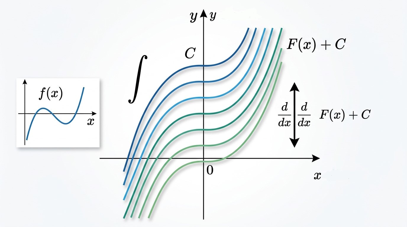
Because the derivative of any constant is zero, adding or subtracting any constant to our function does not change its derivative. This means there are infinitely many antiderivatives for any given function. To represent this entire family of functions, we use the constant of integration, denoted by the letter C.

Thus, the general antiderivative of 2x is written as:

F(x) = x2 + C

Where C is any real number. Geometrically, adding C shifts the graph of the function vertically up or down. All of these shifted curves have the exact same slope at any given value of x, which is why they all share the same derivative function.

Notation: The Indefinite Integral

The process of finding antiderivatives is called antidifferentiation or integration. The mathematical notation used to represent the general antiderivative of a function is the indefinite integral symbol:

∫ f(x) dx = F(x) + C

In this notation:

• ∫ is the integral sign (an elongated "S", standing for "sum").

• f(x) is called the integrand (the function we want to find the antiderivative of).

• dx is the differential, which indicates that x is the variable of integration.

• F(x) + C is the general antiderivative.

Fundamental Rules of Antidifferentiation

Just as there are rules for finding derivatives (like the Power Rule, Product Rule, and Chain Rule), there are corresponding rules for finding antiderivatives. Here are some of the most essential rules that every student must know:

1. The Power Rule for Integration: For any real number n ≠ -1,
   ∫ xn dx = (xn+1 / (n + 1)) + C

2. The Constant Multiple Rule: If k is a constant,
   ∫ k · f(x) dx = k · ∫ f(x) dx

3. The Sum and Difference Rule:
   ∫ [f(x) ± g(x)] dx = ∫ f(x) dx ± ∫ g(x) dx

4. Exponential Functions:
   ∫ ex dx = ex + C

5. The Natural Logarithmic Rule: For x ≠ 0,
   ∫ (1/x) dx = ln|x| + C

6. Trigonometric Functions:
   ∫ cos(x) dx = sin(x) + C
   ∫ sin(x) dx = -cos(x) + C

Physical and Scientific Applications

Antiderivatives are not just abstract mathematical puzzles; they are essential for describing the physical universe. One of the most common applications of antiderivatives is in classical mechanics (kinematics).

1. Moving from Acceleration to Position

In physics, the relationship between position, velocity, and acceleration is defined by derivatives:

• Velocity v(t) is the derivative of position s(t) with respect to time: v(t) = s'(t).

• Acceleration a(t) is the derivative of velocity v(t) with respect to time: a(t) = v'(t).

If we know the acceleration of an object, we can use antiderivatives to work backward and find its velocity and position. Let's look at a real-world example of an object in free fall under the influence of gravity.

Near the surface of the Earth, the acceleration due to gravity is constant, roughly a(t) = -9.8 m/s2 (the negative sign indicates downward acceleration). To find the velocity function, we take the antiderivative of the acceleration function:

v(t) = ∫ a(t) dt = ∫ -9.8 dt = -9.8t + C1

Here, the constant of integration C1 represents the initial velocity of the object, which we usually write as v0. So, v(t) = -9.8t + v0.

To find the position function s(t), we take the antiderivative of the velocity function:

s(t) = ∫ v(t) dt = ∫ (-9.8t + v0) dt = -4.9t2 + v0t + C2

In this step, the new constant of integration C2 represents the initial position of the object, typically written as s0. This gives us the famous kinematic equation used in physics classrooms worldwide:

s(t) = -4.9t2 + v0t + s0

Antiderivatives vs. Definite Integrals

It is common for students to confuse antiderivatives (indefinite integrals) with definite integrals. While they are closely related, they are conceptually distinct:

• An antiderivative (indefinite integral) is a family of functions. It does not have limits of integration and always includes the constant C.

• A definite integral, written with upper and lower limits as ∫ab f(x) dx, represents a specific numerical value (often corresponding to the net area under the curve of the function between x = a and x = b).

The connection between these two concepts is established by the Fundamental Theorem of Calculus. This theorem states that if F is any antiderivative of a continuous function f, then:

∫ab f(x) dx = F(b) - F(a)

This elegant relationship allows us to calculate the exact area under a curve simply by finding the antiderivative of the function and evaluating it at the boundaries.

Key Takeaways

• An antiderivative of a function f(x) is another function F(x) whose derivative is equal to f(x).

• Because the derivative of a constant is zero, every function has an infinite family of antiderivatives, represented by adding the constant of integration, + C.

• Antidifferentiation is denoted by the indefinite integral symbol: ∫ f(x) dx.

• The concept of antiderivatives is vital in physics for reconstructing physical paths (velocity, position) from rates of change (acceleration).

• The Fundamental Theorem of Calculus links antiderivatives directly to definite integrals, making it possible to calculate complex areas and accumulations easily.