How do we find the exact area under a sweeping curve, or calculate the total distance traveled by an accelerating vehicle? The answer lies in a brilliant mathematical concept known as the Riemann sum.
Named after the influential German mathematician Bernhard Riemann (1826–1866), a Riemann sum is a methodical way of approximating the total area under a curve on a graph. By breaking down a complex, curved region into several simple rectangles, we can estimate its area with surprising accuracy. As we increase the number of these rectangles to infinity, this approximation transforms into the exact mathematical value known as the definite integral. In this comprehensive guide, we will explore the intuition, mathematical formulation, types, and real-world applications of Riemann sums.
The Core Intuition: From Rectangles to Curves
Imagine you are asked to paint a wall with a curved top edge. To buy the correct amount of paint, you need to know the area of this wall. Since there is no standard formula for a shape with a curved top, you might decide to divide the wall into several thin, vertical strips. If you treat the top of each strip as a flat, horizontal line instead of a curve, each strip becomes a simple rectangle.
Calculating the area of a rectangle is straightforward: Area = width × height. By summing the areas of all these individual rectangles, you get a solid estimate of the total area of the wall. This is the fundamental philosophy of a Riemann sum. It replaces a continuous, difficult-to-measure curve with a series of discrete, easy-to-measure rectangular bars.
Key Insight: The narrower we make the rectangles, the closer their tops will align with the actual curve, and the more accurate our total area approximation will become.
The Mathematical Definition of a Riemann Sum
To understand Riemann sums rigorously, we must look at how mathematicians define this process using formal notation. Let us break down the components step-by-step.
1. The Interval and Partition
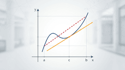
Suppose we have a continuous function f(x) defined over a closed interval [a, b] on the x-axis. We want to estimate the area bounded by the curve, the x-axis, and the vertical lines x = a and x = b.
First, we divide (or "partition") the interval [a, b] into n smaller subintervals. We label the boundary points of these subintervals as:
a = x0 < x1 < x2 < ... < xn = b
2. Width of the Subintervals (Δx)
For simplicity, we often divide the interval into subintervals of equal width. The width of each rectangle, denoted by Δx (delta x), is calculated as:
Δx = (b - a) / n
3. Choosing the Sample Points
To find the height of each rectangle, we must choose a representative x-value within each subinterval. Let us call the sample point in the i-th subinterval xi*. The height of the i-th rectangle will be the value of the function at this point, which is f(xi*).
4. The Summation Formula
The area of a single rectangle is its height multiplied by its width: f(xi*) · Δx. To find the total approximated area, we sum the areas of all n rectangles. Using sigma (Σ) notation, the Riemann sum is written as:
Riemann Sum = ∑i=1n f(xi*) Δx
Types of Riemann Sums
Depending on how we choose the sample points (xi*) within each subinterval, we can construct different types of Riemann sums. The three most common types are:
Left Riemann Sum (Left Endpoint Approximation): We choose the left boundary of each subinterval as our sample point. For the i-th subinterval [xi-1, xi], we set xi* = xi-1.
Right Riemann Sum (Right Endpoint Approximation): We choose the right boundary of each subinterval. For the i-th subinterval, we set xi* = xi.
Midpoint Riemann Sum: We choose the exact middle of each subinterval. This often yields a much more balanced and accurate approximation because the overestimations and underestimations tend to cancel each other out.
A Step-by-Step Numerical Example
Let us walk through a concrete example to see how these approximations work in practice. We want to estimate the area under the curve f(x) = x2 from x = 0 to x = 2 using n = 4 subintervals.
Step 1: Calculate the Width (Δx)
Using our formula with a = 0, b = 2, and n = 4:
Δx = (2 - 0) / 4 = 0.5
Our four subintervals are: [0, 0.5], [0.5, 1.0], [1.0, 1.5], and [1.5, 2.0].
Step 2: Calculate the Left Riemann Sum
For the Left Sum, we evaluate the function at the left endpoints: 0, 0.5, 1.0, and 1.5.
f(0) = 02 = 0
f(0.5) = (0.5)2 = 0.25
f(1.0) = (1.0)2 = 1.0
f(1.5) = (1.5)2 = 2.25
Now, we sum these values and multiply by Δx:
Left Sum = Δx [f(0) + f(0.5) + f(1.0) + f(1.5)]
Left Sum = 0.5 [0 + 0.25 + 1.0 + 2.25] = 0.5 [3.5] = 1.75
Step 3: Calculate the Right Riemann Sum
For the Right Sum, we evaluate the function at the right endpoints: 0.5, 1.0, 1.5, and 2.0.
f(0.5) = 0.25
f(1.0) = 1.0
f(1.5) = 2.25
f(2.0) = (2.0)2 = 4.0
Right Sum = Δx [f(0.5) + f(1.0) + f(1.5) + f(2.0)]
Right Sum = 0.5 [0.25 + 1.0 + 2.25 + 4.0] = 0.5 [7.5] = 3.75
Step 4: Calculate the Midpoint Riemann Sum
For the Midpoint Sum, we find the midpoints of our subintervals: 0.25, 0.75, 1.25, and 1.75.
f(0.25) = (0.25)2 = 0.0625
f(0.75) = (0.75)2 = 0.5625
f(1.25) = (1.25)2 = 1.5625
f(1.75) = (1.75)2 = 3.0625
Midpoint Sum = Δx [f(0.25) + f(0.75) + f(1.25) + f(1.75)]
Midpoint Sum = 0.5 [0.0625 + 0.5625 + 1.5625 + 3.0625] = 0.5 [5.25] = 2.625
Analyzing the Results
Because the function f(x) = x2 is strictly increasing on the interval [0, 2], the Left Sum (1.75) underestimated the true area, while the Right Sum (3.75) overestimated it. The Midpoint Sum (2.625) fell right in between.
Using calculus, we can determine that the exact area under this curve is exactly 8/3 ≈ 2.667. Notice how remarkably close our simple 4-rectangle Midpoint Sum (2.625) is to the absolute truth!
From Riemann Sums to the Definite Integral
The magic of calculus happens when we transition from approximations to exact values. If four rectangles give us a rough estimate, what happens if we use 100 rectangles? What about 10,000? Or a million?
As the number of subintervals n approaches infinity (∞), the width of each rectangle Δx shrinks toward zero. The gap between our rectangular approximation and the true curve vanishes entirely. This infinite limit of a Riemann sum is the formal definition of the definite integral:
∫ab f(x) dx = limn → ∞ ∑i=1n f(xi*) Δx
This equation bridges the gap between discrete summation and continuous integration, forming the bedrock of modern mathematical analysis.
Scientific and Physical Applications
Calculating Distance from Velocity: If an object travels at a constant speed, finding the distance is easy (distance = speed × time). But if a rocket is accelerating dynamically, its speed changes every millisecond. By using a Riemann sum to multiply tiny intervals of time by the rocket's instantaneous velocity, physicists can compute the exact total distance traveled.
Calculating Work Done by Variable Forces: In physics, work is defined as force multiplied by displacement. If the force changes as an object moves (such as stretching a spring), we must sum the work done over tiny increments of distance using Riemann sums.
Hydrostatic Pressure and Center of Mass: Engineers use these sums to calculate the total force exerted by water against dams, or to find the balance point (center of mass) of complex, non-uniform physical structures.
Key Takeaways
A Riemann sum is an approximation tool: It estimates the area under a curve by dividing it into simpler rectangular shapes.
Choice of endpoints matters: Left, right, and midpoint sums yield different approximations, with midpoints generally offering the highest accuracy for a low number of divisions.
It is the foundation of integration: Taking the limit of a Riemann sum as the number of rectangles approaches infinity yields the exact definite integral.
It connects math to reality: Any physical quantity that accumulates over time or space can be modeled and solved using the logic of Riemann sums.