The tool we use to solve this geometric puzzle is the definite integral. Whether you are a physics student calculating the work done by a variable force, an engineer determining the structural load on a bridge, or a calculus student preparing for an exam, understanding how to calculate the area under a curve using definite integrals is a foundational milestone. This comprehensive guide will walk you through the conceptual foundations, the mathematical machinery, and practical step-by-step examples of this elegant process.
The Conceptual Foundation: From Rectangles to Limits
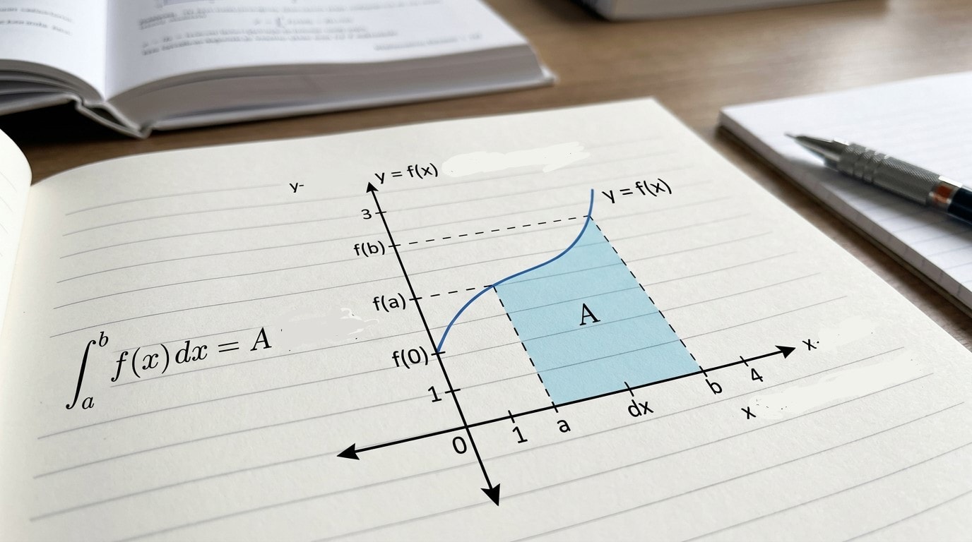
Before diving into the algebraic formulas, it is crucial to understand what "the area under a curve" actually means. Imagine a continuous, non-negative function f(x) plotted on a Cartesian coordinate system. We want to find the area of the region bounded by the curve y = f(x), the x-axis, and the vertical lines x = a and x = b.
How do we measure this area if the top boundary is curved? We begin by approximating it using a shape we know perfectly: the rectangle.
1. Riemann Sums
To approximate the area, we can divide the interval [a, b] into n smaller subintervals, each of equal width, which we denote as Δx (delta x). The width of each subinterval is calculated as:
Δx = (b - a) / n
Over each subinterval, we erect a vertical rectangle. The height of each rectangle is determined by the value of the function f(x) at a chosen point within that subinterval. Depending on where we select this point, we get different types of approximations:
Left Riemann Sum: The height is determined by the function's value at the left endpoint of each subinterval.
Right Riemann Sum: The height is determined by the function's value at the right endpoint of each subinterval.
Midpoint Riemann Sum: The height is determined by the function's value at the exact midpoint of each subinterval.
The total area of these n rectangles is the sum of their individual areas (height multiplied by width):
Approximate Area ≈ f(x1)Δx + f(x2)Δx + ... + f(xn)Δx = Σi=1n f(xi)Δx
2. Taking the Limit to Infinity
If we use only 4 or 5 wide rectangles, our approximation will be quite crude, leaving out gaps or overestimating the curve. However, if we increase the number of rectangles (n) to 50, 500, or 5,000, the rectangles become incredibly thin, and the gaps between the tops of the rectangles and the actual curve virtually disappear.
To find the exact area, we take the mathematical limit as the number of rectangles n approaches infinity (which means the width of each rectangle, Δx, approaches zero):
Exact Area = limn → ∞ Σi=1n f(xi)Δx
This infinite limit of a Riemann sum is precisely the definition of the definite integral. We write this mathematically as:
∫ab f(x) dx
Here, the integration symbol (∫) is an elongated "S" representing a sum, a and b are the lower and upper limits of integration, f(x) represents the height of our infinitely thin rectangles, and dx represents their infinitely small width.
The Fundamental Theorem of Calculus: The Bridge to Evaluation
Calculating limits of infinite sums manually is incredibly tedious and often practically impossible. Fortunately, the Fundamental Theorem of Calculus (FTC) provides an elegant shortcut. It connects the concept of integration (finding areas) with the concept of differentiation (finding rates of change/derivatives).
The second part of the Fundamental Theorem of Calculus states that if a function f(x) is continuous on the interval [a, b], and F(x) is any antiderivative of f(x) (meaning F'(x) = f(x)), then:
∫ab f(x) dx = F(b) - F(a)
This is a profound realization: to find the area under a curve, you do not need to sum up infinite rectangles. You simply need to find the antiderivative of the function, plug in the upper boundary, plug in the lower boundary, and subtract the two values.
Step-by-Step Guide to Calculating the Area
To successfully calculate the area under a curve, follow this systematic four-step process:
Identify the function and the boundaries: Determine the equation of the curve y = f(x) and the interval [a, b] over which you want to find the area.
Set up the definite integral: Write the expression in the standard form: ∫ab f(x) dx.
Find the general antiderivative: Find the antiderivative F(x) of the integrand f(x). Remember, when evaluating a definite integral, you do not need to write the constant of integration (+C), because it cancels out during subtraction.
Evaluate the limits: Calculate F(b) and F(a), and then subtract: F(b) - F(a). The resulting number is the exact area.
A Standard Example: A Polynomial Curve
Let's put this theory into practice with a concrete example. Suppose we want to calculate the area under the quadratic curve f(x) = x2 from x = 1 to x = 3.
Step 1: Set up the Integral
The lower limit is a = 1, and the upper limit is b = 3. Our integral is:
∫13 x2 dx
Step 2: Find the Antiderivative
Using the power rule for integration, which states that ∫ xn dx = (xn+1) / (n+1), we find the antiderivative of x2:
F(x) = x3 / 3
Step 3: Evaluate the Integral
Now we evaluate this antiderivative at our boundaries, 3 and 1:
First, plug in the upper limit (3):
F(3) = 33 / 3 = 27 / 3 = 9
Next, plug in the lower limit (1):
F(1) = 13 / 3 = 1/3
Finally, subtract the lower evaluation from the upper evaluation:
Area = F(3) - F(1) = 9 - 1/3 = 27/3 - 1/3 = 26/3 (or approximately 8.67 square units)
The exact area under the curve y = x2 between x = 1 and x = 3 is exactly 26/3 square units.
Crucial Nuance: Area vs. Net Signed Area
One of the most common pitfalls when learning integration is confusing the definite integral with the physical geometric area. They are not always the same thing.
The definite integral calculates net signed area. This means:
Any region where the curve is above the x-axis (f(x) > 0) is counted as positive area.
Any region where the curve is below the x-axis (f(x) < 0) is counted as negative area.
If you evaluate a definite integral over an interval where the function goes both above and below the x-axis, the positive and negative regions will cancel each other out. If they are perfectly symmetrical, the definite integral will evaluate to zero, even though there is clearly physical area present.
How to Find the Total Physical Area
If a question asks for the total physical area bounded by a curve that crosses the x-axis, you must follow these extra steps:
Find the x-intercepts of the function within your interval by setting f(x) = 0 and solving for x.
Divide the original interval into subintervals based on these intercepts.
Integrate the function over each subinterval separately.
Take the absolute value of each result (turning negative areas positive) and add them together.
Advanced Example: A Curve Crossing the X-Axis
Let us calculate the total physical area bounded by the curve f(x) = x3 - 4x and the x-axis over the interval [-2, 2].
Step 1: Find the X-Intercepts
First, let's find where the curve crosses the x-axis by setting the function to zero:
x3 - 4x = 0
x(x2 - 4) = 0
x(x - 2)(x + 2) = 0
The roots are x = -2, x = 0, and x = 2. All of these lie within our interval [-2, 2]. Therefore, our curve crosses the x-axis at x = 0, splitting our interval into two sections: [-2, 0] and [0, 2].
Step 2: Set Up the Separate Integrals
We must set up two separate definite integrals:
Area 1 = ∫-20 (x3 - 4x) dx
Area 2 = ∫02 (x3 - 4x) dx
Step 3: Integrate and Evaluate
The general antiderivative of x3 - 4x is:
F(x) = x4 / 4 - 2x2
Evaluating Area 1 (from -2 to 0):
F(0) = 04/4 - 2(0)2 = 0
F(-2) = (-2)4/4 - 2(-2)2 = 16/4 - 2(4) = 4 - 8 = -4
Area 1 = F(0) - F(-2) = 0 - (-4) = 4
Evaluating Area 2 (from 0 to 2):
F(2) = 24/4 - 2(2)2 = 16/4 - 2(4) = 4 - 8 = -4
F(0) = 0
Area 2 = F(2) - F(0) = -4 - 0 = -4
Step 4: Sum the Absolute Values
If we had integrated straight from -2 to 2, the result would have been 4 + (-4) = 0. However, the physical area is the sum of the absolute values of the individual regions:
Total Physical Area = |Area 1| + |Area 2| = |4| + |-4| = 4 + 4 = 8 square units
By splitting the integral at the root, we correctly determined that the total physical area under (and over) the curve is 8 square units.
Scientific and Physical Applications
Kinematics (Distance Traveled): If you plot an object's velocity over time, the area under that velocity-time curve represents the total displacement of the object. When velocity fluctuates, integration is the only way to find the exact distance traveled.
Physics (Work Done): In physics, work is defined as force multiplied by displacement. If the force applied to an object changes as it moves (like stretching a spring), the work done is calculated as the area under the force-displacement curve: W = ∫ F(x) dx.
Probability (Statistics): In continuous probability distributions (such as the bell curve or normal distribution), the total area under the probability density curve is always equal to 1. The probability of an event occurring within a specific range [a, b] is found by calculating the definite integral of the probability density function over that range.
Key Takeaways
Calculating the area under a curve is one of the most powerful applications of calculus. Here are the core concepts to remember:
The Definite Integral represents the limit of an infinite sum of rectangular approximations (Riemann Sums) as their widths approach zero.
The Fundamental Theorem of Calculus allows us to bypass infinite sums by using antiderivatives: ∫ab f(x) dx = F(b) - F(a).
Net Signed Area vs. Total Area: Standard definite integrals subtract areas below the x-axis from areas above it. To find the physical, geometric area, you must locate x-intercepts, split the integration intervals, and sum the absolute values of the individual components.