Real-world scenarios are the direct, physical application of one of the most fundamental principles in mathematical analysis: The Mean Value Theorem (MVT). Often hailed as the gateway to modern calculus, the Mean Value Theorem bridges the gap between an average rate of change and an instantaneous rate of change. In this comprehensive guide, we will explore the historical foundations, mathematical formulations, geometric interpretations, rigorous proofs, and profound scientific consequences of this elegant theorem.
The Mathematical Foundation: Rolle's Theorem
To fully comprehend the Mean Value Theorem, we must first examine its historical and logical precursor: Rolle's Theorem. Named after the French mathematician Michel Rolle, who stated it in 1691, this theorem addresses a specific, simplified case of the Mean Value Theorem.
Rolle's Theorem states that if a real-valued function f satisfies three specific conditions:
It is continuous on the closed interval [a, b].
It is differentiable on the open interval (a, b).
The function values at the endpoints are equal, meaning f(a) = f(b).
Then, there must exist at least one number c in the open interval (a, b) such that the derivative at that point is zero:
f'(c) = 0
Geometrically, this means that if a smooth curve starts and ends at the exact same height, there must be at least one point between the endpoints where the curve stops rising or falling and flattens out. At this point, the tangent line to the curve is perfectly horizontal.
Stating the Mean Value Theorem
The Mean Value Theorem, first formulated in its modern form by the legendary mathematician Joseph-Louis Lagrange, generalizes Rolle's Theorem by removing the constraint that the endpoint values must be equal (f(a) = f(b)). It allows the endpoints to be at different heights, tilting the entire scenario.
The formal statement of the Mean Value Theorem is as follows:
Let f be a function that satisfies the following two hypotheses:
f is continuous on the closed interval [a, b].
f is differentiable on the open interval (a, b).
Then, there exists at least one number c in the open interval (a, b) such that:
f'(c) = [f(b) - f(a)] / (b - a)
This simple equation is incredibly powerful. Let's break down what each side represents:
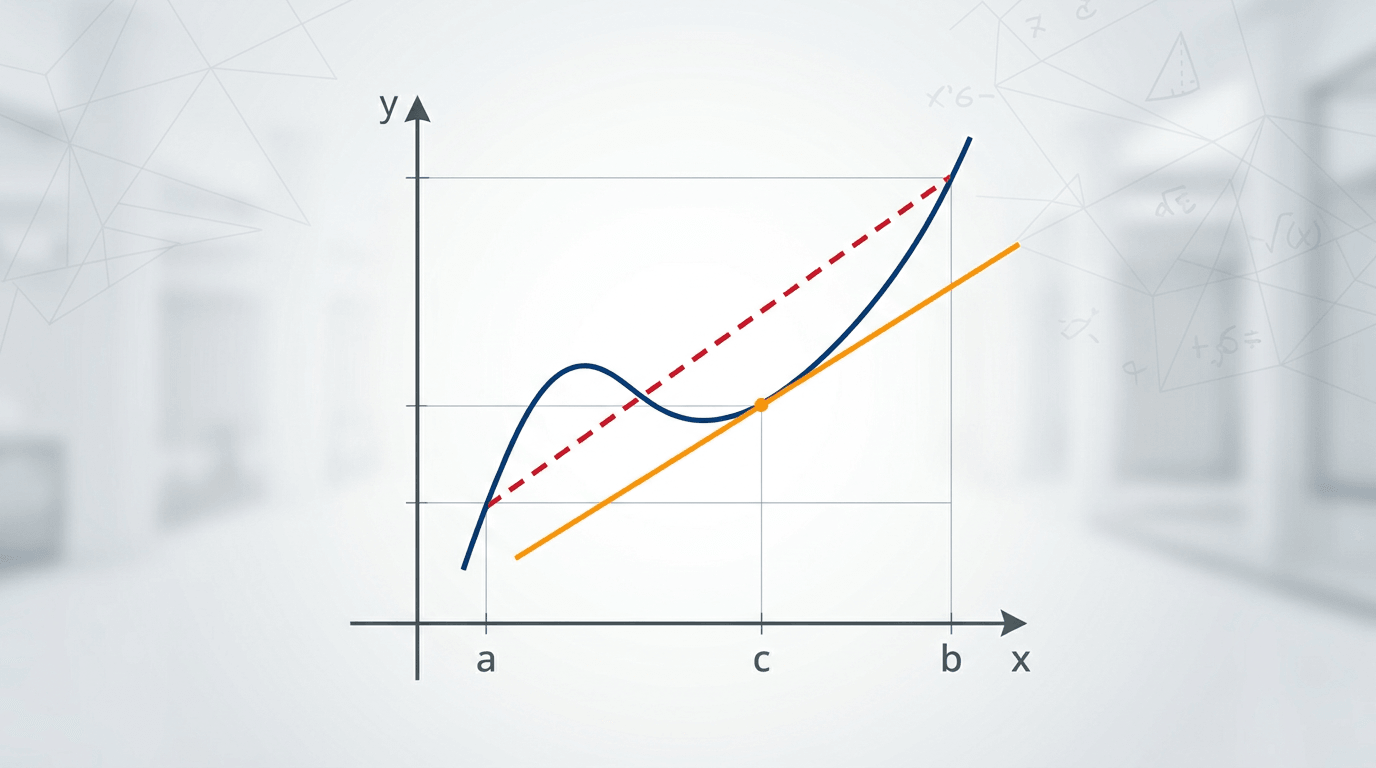
[f(b) - f(a)] / (b - a) is the average rate of change of the function over the interval [a, b]. Geometrically, this is the slope of the secant line connecting the two endpoint coordinates (a, f(a)) and (b, f(b)).
f'(c) is the instantaneous rate of change of the function at the specific point c. Geometrically, this is the slope of the tangent line to the curve at the point (c, f(c)).
Therefore, the Mean Value Theorem guarantees that there is at least one point on the curve where the instantaneous rate of change equals the average rate of change. Geometrically, it asserts that there is a point where the tangent line is parallel to the secant line.
The Geometric Interpretation
To visualize the Mean Value Theorem, plot a smooth, unbroken curve on a coordinate grid from an starting point A to an ending point B. Draw a straight line directly connecting A and B; this is your secant line. The slope of this line represents the average speed, average growth, or average rate of change over the entire journey.
Now, imagine sliding this straight secant line upwards or downwards while keeping its slope exactly the same (parallel to the original line). As long as the curve is smooth and continuous, the parallel line will eventually touch the curve at one or more points without crossing it. At these points of contact, the parallel line acts as a tangent line. The x-coordinate of any such point of tangency is our value c. The derivative at c is identical to the slope of our original secant line.
A Rigorous Mathematical Proof
How do we prove this theorem? We can do so by constructing an auxiliary function and applying Rolle's Theorem. The goal is to measure the vertical distance between the curve f(x) and the secant line connecting the endpoints.
First, let us write the equation of the secant line passing through (a, f(a)) and (b, f(b)) using the point-slope form:
y - f(a) = ([f(b) - f(a)] / (b - a)) * (x - a)
Solving for y gives the equation of the line:
y = f(a) + ([f(b) - f(a)] / (b - a)) * (x - a)
Now, we define a new auxiliary function, h(x), which represents the vertical difference between the curve and this secant line at any point x:
h(x) = f(x) - [f(a) + ([f(b) - f(a)] / (b - a)) * (x - a)]
Let us verify if h(x) satisfies the conditions of Rolle's Theorem:
Continuity: Since f(x) is continuous on [a, b] and the linear part is also continuous everywhere, h(x) is continuous on [a, b].
Differentiability: Since f(x) is differentiable on (a, b) and the linear part is differentiable everywhere, h(x) is differentiable on (a, b).
Endpoint values: Let's evaluate h(x) at the boundaries a and b:
h(a) = f(a) - [f(a) + 0] = 0
h(b) = f(b) - [f(a) + (f(b) - f(a))] = f(b) - f(b) = 0
Thus, h(a) = h(b) = 0.
Because h(x) satisfies all three hypotheses of Rolle's Theorem, there must exist some number c in (a, b) such that the derivative h'(c) = 0.
Let us find the derivative of h(x):
h'(x) = f'(x) - [f(b) - f(a)] / (b - a)
Setting h'(c) = 0 yields:
0 = f'(c) - [f(b) - f(a)] / (b - a)
Which simplifies directly to:
f'(c) = [f(b) - f(a)] / (b - a)
This completes the proof of the Mean Value Theorem.
The Crucial Importance of the Hypotheses
A common pitfall for students is applying the Mean Value Theorem without verifying its strict conditions. If either continuity on the closed interval or differentiability on the open interval is violated, the theorem's conclusion can fail completely.
Counterexample 1: Lack of Differentiability
Consider the absolute value function f(x) = |x| on the interval [-1, 1].
The function is continuous on [-1, 1].
The average rate of change is: [f(1) - f(-1)] / (1 - (-1)) = [1 - 1] / 2 = 0.
However, there is no point c in (-1, 1) where f'(c) = 0. The derivative is -1 for negative values and 1 for positive values. At x = 0, the function has a sharp corner (clash of limits) and is not differentiable.
Because the function is not differentiable on the entire open interval (-1, 1), the Mean Value Theorem does not apply, and indeed, no such c exists.
Counterexample 2: Lack of Continuity
Consider a step function g(x) defined on [0, 2] such that g(x) = x for 0 ≤ x < 1, and g(x) = x + 2 for 1 ≤ x ≤ 2.
The average rate of change over [0, 2] is: [g(2) - g(0)] / (2 - 0) = [4 - 0] / 2 = 2.
The derivative g'(x) is equal to 1 everywhere except at the jump discontinuity x = 1.
There is no point where the derivative equals the average rate of change of 2.
Because the function is discontinuous at x = 1, the theorem fails. These examples highlight why checking mathematical conditions is not a mere formality, but an absolute necessity.
Profound Consequences and Applications
While the Mean Value Theorem is beautiful geometrically, its true power lies in the theoretical machinery it provides. It is used to prove many of the core rules of calculus that we take for granted.
1. Determining Monotonicity (Increasing and Decreasing Functions)
How do we mathematically prove that a positive derivative means a function is increasing? We use the Mean Value Theorem. Suppose f'(x) > 0 on an interval. Let x1 and x2 be any two points in the interval such that x1 < x2. Applying the MVT to the interval [x1, x2], we get:
f(x2) - f(x1) = f'(c) * (x2 - x1)
Since f'(c) > 0 and (x2 - x1) > 0, the product must be positive. Therefore, f(x2) - f(x1) > 0, which means f(x2) > f(x1). This rigorously proves that the function is strictly increasing.
2. The Constant Function Theorem
If a car's speedometer reads exactly 0 mph for an entire hour, the car has not moved. Mathematically, if f'(x) = 0 for all x in an interval, then the function must be constant. The proof relies directly on the MVT, showing that for any two points x1 and x2, f(x2) - f(x1) = 0 * (x2 - x1) = 0, meaning f(x1) = f(x2).
3. Uniqueness of Antiderivatives
A direct corollary of the Constant Function Theorem is that if two functions have the exact same derivative on an interval (f'(x) = g'(x)), then they must differ only by a constant: f(x) = g(x) + C. This is the foundational justification for adding the constant of integration "+ C" in indefinite integrals.
Key Takeaways
The Core Concept: The Mean Value Theorem states that for a sufficiently smooth curve, there is at least one point where the instantaneous rate of change (tangent slope) equals the average rate of change (secant slope) over an interval.
The Requirements: The function must be continuous on the closed interval [a, b] and differentiable on the open interval (a, b). If these conditions are not met, the theorem cannot guarantee any results.
The Precursor: Rolle's Theorem is a special case of the MVT where the endpoints have the same height, resulting in a point with a horizontal tangent line (slope of zero).
The Impact: MVT is not just a theoretical concept; it is the mathematical backbone used to prove rules regarding increasing/decreasing functions, local extrema, and the fundamental structures of integral calculus.