In the study of calculus, the concept of a limit is the foundation upon which derivatives, integrals, and continuity are built. When we talk about limits, we are interested in understanding how a function behaves as its input gets closer and closer to a specific value. However, functions can sometimes behave erratically or exhibit sudden jumps. To analyze these complex behaviors with precision, mathematicians split the concept of a limit into two directions: the left-hand limit and the right-hand limit. In this comprehensive guide, we will dive deep into the concept of the right-hand limit, exploring its definition, mathematical representation, graphical interpretation, and real-world scientific applications.
Understanding the Core Concept
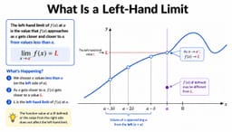
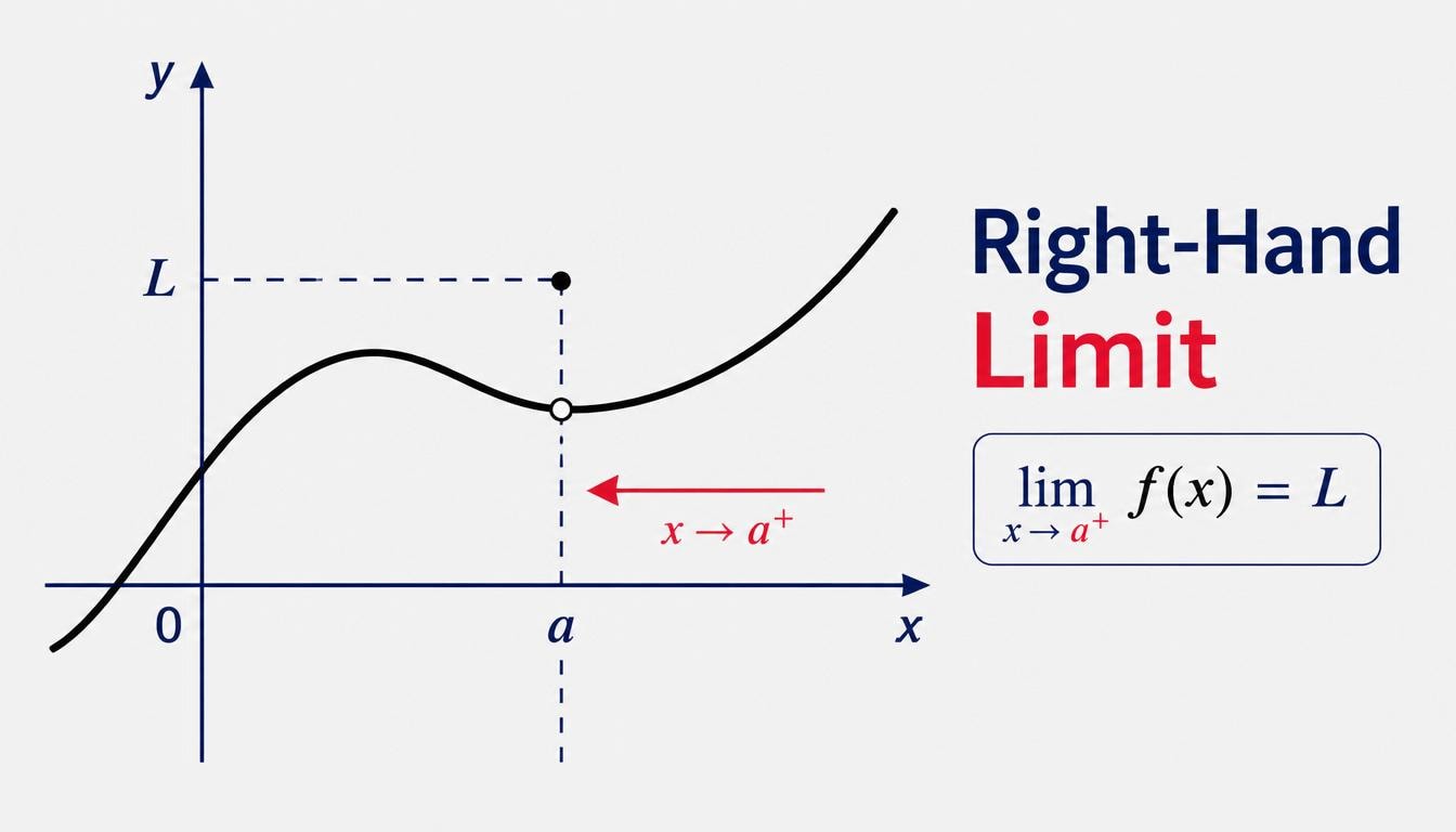
To understand a right-hand limit, imagine you are walking along the graph of a function from right to left, moving toward a specific target x-value. As you walk along this path, you observe the height (the y-value) of the graph. The value that your height approaches as you get infinitely close to the target x-value from the right side is called the right-hand limit.
The crucial detail here is the direction of approach. We are strictly looking at values of x that are greater than the target value. We do not care about what is happening on the left side of the target, nor do we necessarily care about the actual value of the function at the target point itself. We only care about the trend of the function as we approach from the right.
The Mathematical Notation
In mathematical notation, the right-hand limit is written using a small plus sign (+) as a superscript next to the target value. This superscript does not mean the number is positive; rather, it indicates the direction of approach (from the positive or right side of the number line).
Mathematical Definition:
We write:
lim (x → a⁺) f(x) = L
This is read as: "The limit of f(x) as x approaches a from the right is equal to L." This means that we can make the values of f(x) as close to L as we want by choosing x to be sufficiently close to a, with x always being strictly greater than a.
A Numerical Example
Let us look at a numerical example to make this concrete. Consider a piecewise-defined function f(x) that behaves differently on either side of x = 3:
f(x) = 2x + 1, for x ≥ 3
f(x) = x - 2, for x < 3
Suppose we want to find the right-hand limit of f(x) as x approaches 3. Because we are looking at the right-hand limit, we must choose values of x that are slightly larger than 3 and getting closer to 3. Let us construct a table of values:
For x = 3.1: f(3.1) = 2(3.1) + 1 = 7.2
For x = 3.01: f(3.01) = 2(3.01) + 1 = 7.02
For x = 3.001: f(3.001) = 2(3.001) + 1 = 7.002
For x = 3.0001: f(3.0001) = 2(3.0001) + 1 = 7.0002
As you can see, as the values of x get closer and closer to 3 from the right side (3.1, 3.01, 3.001...), the output values of the function get closer and closer to 7. Therefore, we can confidently state that:
lim (x → 3⁺) f(x) = 7
Notice that if we had approached from the left side (using values like 2.9, 2.99, etc.), we would have used the other part of the formula (x - 2), which would lead us to a completely different value (1). This highlights why specifying the direction of the limit is so important.
Graphical Interpretation of Right-Hand Limits
Visualizing limits graphically is often the easiest way to master the concept. Imagine a graph with a physical break or a "jump" at a certain point, say x = c. To find the right-hand limit at x = c:
Locate the value c on the horizontal x-axis.
Place your pencil on the curve to the right of x = c.
Trace the curve to the left, moving toward the vertical line x = c.
Look at the y-value your pencil is pointing to as you reach the line x = c. That y-value is your right-hand limit.
Even if there is an open circle (a hole) at that point on the graph, or if the actual point is plotted somewhere else entirely, the right-hand limit remains the value that the curve is pointing to from the right side.
The Relationship Between One-Sided Limits and General Limits
One-sided limits (both left-hand and right-hand limits) are the building blocks of the general, two-sided limit. A fundamental theorem in calculus describes this relationship:
The general limit of f(x) as x approaches a exists and is equal to L if and only if both the left-hand limit and the right-hand limit exist and are equal to L.
In logical terms:
lim (x → a) f(x) = L ⇔ lim (x → a⁻) f(x) = L and lim (x → a⁺) f(x) = L
If the left-hand limit and the right-hand limit point to different values, we say that the general limit at that point does not exist (DNE). This is common at jump discontinuities, which frequently appear in both pure mathematics and physical applications.
Scientific and Physical Applications
Right-hand limits are not just abstract mathematical constructs; they are vital for modeling real-world phenomena where sudden, instantaneous changes occur. In classical physics and engineering, we often use idealized step functions to represent rapid transitions.
1. Electrical Engineering and Switch States
Consider an electrical circuit with a switch that is flipped on at exactly time t = 0. Before t = 0, the current flowing through the circuit is 0 amperes. At t = 0, the switch closes, and the current instantly jumps to 5 amperes. We can model the current I(t) as a step function:
I(t) = 0, for t < 0
I(t) = 5, for t ≥ 0
If we want to analyze the state of the circuit immediately after the switch is flipped, we look at the right-hand limit as t approaches 0. Mathematically, lim (t → 0⁺) I(t) = 5. This tells engineers the immediate state of the system as time progresses forward from the moment of activation.
2. Classical Mechanics and Sudden Collisions
In physics, when an elastic ball bounces off a hard wall, its velocity changes direction almost instantaneously. If we model this collision as happening at time t = c, the velocity function v(t) has a jump discontinuity. The left-hand limit represents the velocity of the ball immediately before the impact, while the right-hand limit represents the velocity of the ball immediately after the impact. Analyzing the right-hand limit allows physicists to calculate the post-collision trajectory and momentum.
Common Pitfalls to Avoid
When learning about right-hand limits, students often encounter a few common misunderstandings:
Confusing the superscript with signs: The notation x → -2⁺ does not mean we are approaching positive 2. It means we are approaching the negative number -2 from the right side (using values like -1.9, -1.99, -1.999).
Assuming the limit must equal the function value: The right-hand limit as x approaches a can exist even if the function is completely undefined at x = a, or if f(a) is defined as a different value. The limit is about the journey, not the destination.
Key Takeaways
To summarize, here are the most important points to remember about right-hand limits:
A right-hand limit focuses exclusively on how a function behaves as the input approaches a target value from the right side (values greater than the target).
It is denoted by a superscript plus sign: lim (x → a⁺) f(x).
It is highly useful for analyzing piecewise functions, step functions, and graphs with jump discontinuities.
For a general, two-sided limit to exist, the right-hand limit and the left-hand limit must exist and be equal to each other.
Real-world applications include modeling sudden transitions in physics, chemistry, and electrical engineering.