In the study of calculus, the concept of a limit is the cornerstone upon which derivatives, integrals, and continuous functions are built. When we talk about limits, we are asking a fundamental question: What value does a function approach as the input gets closer and closer to a specific number?
However, functions can be complex, unpredictable, and sometimes fractured. To analyze them precisely, mathematicians break the concept of a limit down into directions. This brings us to the concept of one-sided limits. In this comprehensive guide, we will dive deep into one of the most critical foundational concepts of calculus: the left-hand limit.
Understanding the Intuition Behind One-Sided Limits
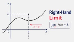
Imagine you are walking along a path on a mountain ridge, and you want to know the altitude of a specific landmark ahead. You can approach this landmark from two directions: from the west (left) or from the east (right). If the path is continuous, both directions will lead you to the exact same altitude. But what if there is a sudden cliff or a vertical step? Approaching from the west might lead you to a low ledge, while approaching from the east might bring you to a high plateau.
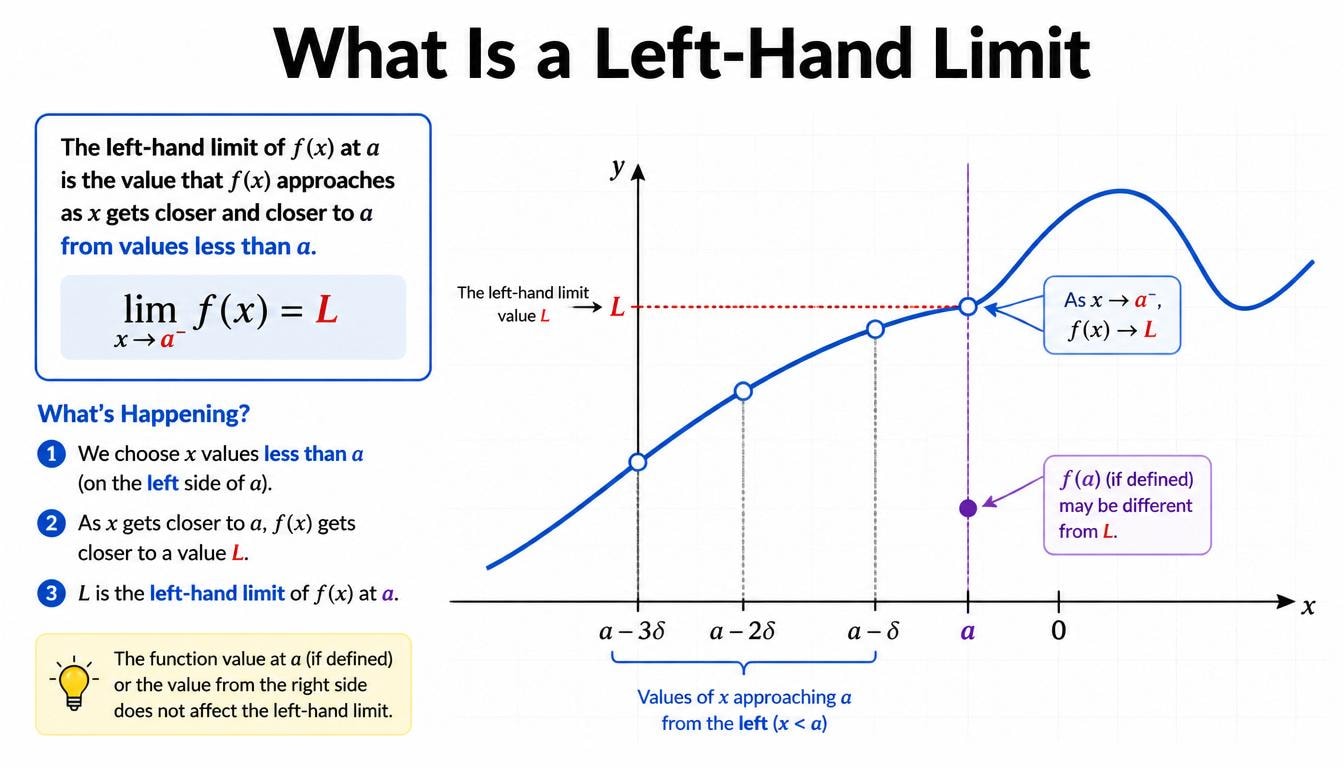
In mathematics, functions can behave exactly like this fractured path. To understand their behavior at a specific point, we must inspect how they behave when we approach that point from only one side. When we approach from the left—using values that are strictly less than our target value—we are finding the left-hand limit.
The Formal Definition of a Left-Hand Limit
Mathematically, we define the left-hand limit as the value that a function f(x) approaches as the independent variable x approaches a specific value c from the left side (meaning x is always less than c).
We express this using the following notation:
limx → c− f(x) = L
In this notation:
lim represents the limit operation.
x → c− indicates that x is approaching the constant c from the left (the minus sign superscript denotes values smaller than c).
f(x) is the function we are analyzing.
L is the unique real number that the function values approach.
Formulating Hypotheses and Observing Patterns
To truly grasp how a left-hand limit works, let us engage in a mathematical exploration. Suppose we have a function:
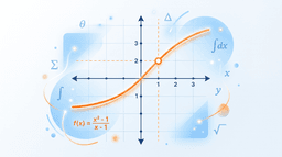
f(x) = (x2 - 1) / (x - 1)
We want to find out what happens to this function as x approaches 1 from the left (x → 1−). Note that if we plug x = 1 directly into the function, we get the indeterminate form 0/0, which is undefined. This is why limits are so powerful—they allow us to explore the behavior of a function where it cannot legally exist.
Step 1: Making a Hypothesis
Before calculating, we can make a hypothesis. Since the numerator can be factored as (x - 1)(x + 1), for all values of x not equal to 1, the function simplifies to f(x) = x + 1. Therefore, we hypothesize that as x gets closer to 1 from the left, f(x) should get closer to 1 + 1 = 2.
Step 2: Listing Patterns with Numerical Data
Let us verify our hypothesis by selecting values of x that are strictly less than 1, moving progressively closer to 1:
For x = 0.9: f(0.9) = (0.92 - 1) / (0.9 - 1) = (0.81 - 1) / (-0.1) = -0.19 / -0.1 = 1.9
For x = 0.99: f(0.99) = (0.992 - 1) / (0.99 - 1) = 1.99
For x = 0.999: f(0.999) = (0.9992 - 1) / (0.999 - 1) = 1.999
For x = 0.9999: f(0.9999) = 1.9999
Step 3: Generalizing the Pattern
By observing this sequence of numbers, a clear pattern emerges. As the input values x get infinitely close to 1 from the left side, the output values f(x) get infinitely close to 2. We can generalize this pattern to state that the left-hand limit of this function at x = 1 is indeed 2:
limx → 1− f(x) = 2
The Crucial Role of Left-Hand Limits in Piecewise Functions
While the previous example was simple, left-hand limits are absolutely essential when dealing with piecewise functions. These are functions defined by different formulas over different intervals.
Consider the following piecewise function:
g(x) =
• x + 3 if x < 2
• x2 - 1 if x ≥ 2
Let us find the left-hand limit of g(x) as x approaches 2. Since we are approaching from the left (x → 2−), we must only look at the domain where x is strictly less than 2. According to our function definition, this means we must use the formula g(x) = x + 3.
Evaluating this limit:
limx → 2− g(x) = limx → 2− (x + 3) = 2 + 3 = 5
Now, let's look at what happens if we approach from the right (x → 2+). For values greater than or equal to 2, we use g(x) = x2 - 1:
limx → 2+ g(x) = limx → 2+ (x2 - 1) = 22 - 1 = 3
Because the left-hand limit (5) and the right-hand limit (3) are not equal, we can make a powerful mathematical proposition.
Mathematical Propositions: Connecting One-Sided Limits to the General Limit
By analyzing various functions and comparing our left-hand and right-hand limits, we can formulate a fundamental theorem of calculus:
Proposition: The general limit of a function f(x) as x approaches c exists if and only if both the left-hand limit and the right-hand limit exist and are equal to the same real number L.
Symbolically, we write:
limx → c f(x) = L ⇔ limx → c− f(x) = L and limx → c+ f(x) = L
In our piecewise function g(x) above, because the left-hand limit was 5 and the right-hand limit was 3, the general limit limx → 2 g(x) does not exist (DNE). This demonstrates why calculating the left-hand limit independently is a critical diagnostic tool in mathematical analysis.
Real-World Applications: The Physics of Left-Hand Limits
Limits are not just abstract symbols on a blackboard; they describe how the physical universe changes over time. Let's look at how left-hand limits apply to real-world scenarios.
1. Instantaneous Velocity
Suppose you are driving a car and suddenly slam on the brakes at exactly t = 3 seconds. If we want to calculate your instantaneous deceleration or speed at exactly t = 3 seconds, we must look at the history of your motion leading up to that moment.
By calculating the limit of your average velocity as time t approaches 3 seconds from the left (from past times like 2.9 seconds, 2.99 seconds, etc.), we are using a physical left-hand limit:
v(3) = limt → 3− [s(3) - s(t)] / (3 - t)
This left-hand limit tells us the exact speed of the car immediately before the braking mechanism altered the vehicle's state of motion.
2. Electrical Engineering and Step Functions
In electrical engineering, when you flip a switch, the voltage in a circuit jumps instantly from 0 volts to 5 volts. This is modeled using the Heaviside step function. If we analyze the voltage V(t) at the exact millisecond the switch is flipped (let's say t = 0):
The left-hand limit limt → 0− V(t) = 0 (the state of the circuit before the action).
The right-hand limit limt → 0+ V(t) = 5 (the state of the circuit immediately after the action).
Here, the left-hand limit represents the physical history of the system, a critical parameter for preventing electrical surges and designing safe circuits.
Key Takeaways
Directional Approach: A left-hand limit focuses exclusively on how a function behaves as the input approaches a target value from the left side (values smaller than the target).
Notation: It is denoted by a minus sign superscript: limx → c− f(x).
Existence of Limits: For a general limit to exist at a point, the left-hand limit and the right-hand limit at that point must be equal.
Physical Significance: Left-hand limits represent the state of physical systems (like velocity or electric current) immediately leading up to a specific moment in time.