Calculus is often described as the mathematics of change. At the heart of this profound branch of mathematics lies a single, revolutionary concept: the limit. Without limits, we would have no derivatives, no integrals, and no way to precisely calculate the instantaneous rate of change of a moving object. But how do we work with limits systematically? Just as arithmetic has rules like addition and multiplication, calculus has a set of fundamental rules known as the properties of limits (or limit laws).
In this comprehensive guide, we will explore these properties in detail. We will move from basic arithmetic rules to the complex scenarios of indeterminate forms like 0/0 and infinity/infinity, formulate hypotheses, test them with patterns, and apply our findings to real-world physics problems like instantaneous velocity.
Understanding the Concept of a Limit
Before diving into the algebraic properties, let us establish what a limit actually is. When we say that the limit of a function f(x) as x approaches a point c is equal to L, we write:
limx → c f(x) = L
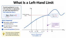
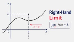
This means that as the input x gets closer and closer to the number c (from both the left and the right sides, without actually reaching c), the output value f(x) gets arbitrarily close to the real number L. The beauty of limits is that they allow us to inspect the behavior of a function at points where the function itself might not even be defined.
The Fundamental Properties of Limits (Limit Laws)
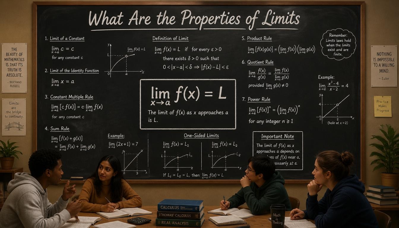
To evaluate limits algebraically without relying on graphs or tables of values every time, mathematicians use several core properties. Let us assume that the limits limx → c f(x) = L and limx → c g(x) = M exist, and that k is a constant.
1. The Sum Rule
The limit of the sum of two functions is the sum of their limits. This allows us to break down complex expressions into simpler parts.
limx → c [f(x) + g(x)] = L + M
2. The Difference Rule
Similarly, the limit of the difference of two functions is the difference of their limits.
limx → c [f(x) - g(x)] = L - M
3. The Constant Multiple Rule
You can pull a constant factor out of a limit.
limx → c [k · f(x)] = k · L
4. The Product Rule
The limit of a product is the product of the individual limits.
limx → c [f(x) · g(x)] = L · M
5. The Quotient Rule
The limit of a quotient is the quotient of the limits, provided that the limit of the denominator is not zero.
limx → c [f(x) / g(x)] = L / M (where M ≠ 0)
6. The Power and Root Rules
For any positive integer n:
limx → c [f(x)]n = Ln
limx → c &supn;√f(x) = &supn;√L (if n is even, L must be positive).
The Challenge of Indeterminate Forms
The properties listed above work beautifully—until we encounter a situation where the quotient rule fails because the denominator limit is zero. Specifically, we often find ourselves facing expressions that yield 0/0 or ∞/∞ when we try direct substitution.
Formulating a Hypothesis
Imagine evaluating the limit of f(x) = (x2 - 4) / (x - 2) as x approaches 2. Direct substitution yields:
f(2) = (22 - 4) / (2 - 2) = 0/0
What does "0/0" mean? Let us make a few intuitive hypotheses:
Hypothesis A: Because any fraction with 0 in the numerator is 0, the limit must be 0.
Hypothesis B: Because division by zero is undefined, the limit does not exist.
Hypothesis C: Because any number divided by itself is 1, the limit must be 1.
Analyzing Patterns to Generalize
To test these hypotheses, let us observe the behavior of different functions that yield 0/0 under direct substitution. We can list different cases and analyze their patterns:
Case 1: Factoring Rational Functions
Let f(x) = (x2 - 4) / (x - 2) as x → 2.
We can factor the numerator: (x - 2)(x + 2) / (x - 2). For all x ≠ 2, we can cancel the (x - 2) term, leaving us with (x + 2).
Now, evaluating the limit: limx → 2 (x + 2) = 4.
Result: 4Case 2: Simplifying Polynomial Powers
Let g(x) = (3x2) / x as x → 0.
Direct substitution yields 0/0. Simplifying the fraction gives us 3x.
Evaluating the limit: limx → 0 3x = 0.
Result: 0Case 3: Radical Expressions and Conjugates
Let h(x) = (√(x + 1) - 1) / x as x → 0.
Direct substitution yields 0/0. Multiplying the numerator and denominator by the conjugate (√(x + 1) + 1) simplifies the function to 1 / (√(x + 1) + 1).
Evaluating the limit: limx → 0 [1 / (√(x + 1) + 1)] = 1/2.
Result: 1/2
Comparing Generalizations with Hypotheses
By analyzing these patterns, we can make a crucial generalization: The indeterminate form 0/0 does not have a fixed value. It can equal 4, 0, 1/2, or indeed any real number depending on the rates at which the numerator and the denominator approach zero. Therefore, our initial hypotheses (that the limit must be 0, 1, or simply not exist) are incorrect. The form 0/0 is "indeterminate" precisely because the limit's value cannot be determined without further algebraic manipulation.
Formulating Mathematical Propositions
From our pattern analysis, we can propose the following mathematical statements:
Proposition 1: If a rational function f(x) = P(x)/Q(x) yields the indeterminate form 0/0 at x = c, then (x - c) is a common factor of both P(x) and Q(x). Simplifying this factor resolves the indeterminacy.
Proposition 2: The limit of an indeterminate quotient represents a struggle between the numerator trying to pull the fraction to zero and the denominator trying to push it to infinity. The final limit is determined by which term approaches its target "faster."
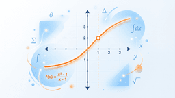
Today, students and scientists do not have to rely solely on manual algebra to verify these propositions. Using dynamic mathematics software like GeoGebra or Desmos, we can plot these functions and visually inspect the "hole" (removable discontinuity) in the graph, confirming that the curve smoothly approaches the exact limit value we calculated algebraically.
Real-World Application: Finding Instantaneous Velocity
Why do we care so much about resolving 0/0 limit properties? The answer lies in physics. The fundamental definition of speed is distance divided by time. But how do we calculate speed at one *exact* instant in time?
If you try to calculate speed at an exact instant, the elapsed time (Δt) is 0, and the distance traveled (Δs) is also 0. This gives us the classic indeterminate form: 0/0.
The Physics Problem
Suppose a falling object's position is given by the function s(t) = 5t2, where s is in meters and t is in seconds. We want to find the instantaneous velocity of the object at exactly t = 2 seconds.
The average velocity over a tiny interval of time Δt is given by:
Average Velocity = [s(2 + Δt) - s(2)] / Δt
To find the instantaneous velocity, we must take the limit as Δt approaches 0:
Instantaneous Velocity = limΔt → 0 [5(2 + Δt)2 - 5(2)2] / Δt
If we directly substitute Δt = 0, we get the indeterminate form 0/0. Let us apply our limit algebraic properties to solve it:
Expand the numerator: 5(4 + 4Δt + (Δt)2) - 20
Simplify: 20 + 20Δt + 5(Δt)2 - 20 = 20Δt + 5(Δt)2
Substitute back into the limit: limΔt → 0 [20Δt + 5(Δt)2] / Δt
Factor out Δt from the numerator: limΔt → 0 [Δt(20 + 5Δt)] / Δt
Cancel the common factor Δt (since Δt ≠ 0): limΔt → 0 (20 + 5Δt)
Apply the Sum Rule and evaluate: 20 + 5(0) = 20 m/s
By resolving the 0/0 limit using algebraic properties, we have successfully calculated that the object is traveling at exactly 20 meters per second at t = 2.
Key Takeaways
Limit Laws provide a reliable, step-by-step algebraic framework to evaluate complex limits without guessing.
Indeterminate forms like 0/0 do not mean a limit does not exist; they indicate that further algebraic work (factoring, conjugates, simplification) is required.
Limits bridge the gap between static algebra and dynamic physics, enabling us to define real-world concepts like instantaneous velocity and acceleration.
Digital tools like graphing software help us visualize these abstract concepts, turning algebraic proofs into intuitive, visual realities.