What are concavity and convexity?

Introduction to Curvature: Beyond Slopes

When we study functions, our first instinct is often to look at whether they are increasing or decreasing. This is determined by the first derivative, which gives us the slope of the tangent line at any given point. However, knowing whether a function is rising or falling is only half the story. To truly understand the behavior of a curve, we must look at how it rises or falls. This is where the concepts of concavity and convexity come into play.

These terms describe the curvature of a graph. They tell us whether a curve is bending upward or downward, which has profound implications in mathematics, physics, economics, and optical science. In this comprehensive guide, we will explore what concavity and convexity mean, how to analyze them mathematically using calculus, and how they manifest in the physical world.

Defining Concavity and Convexity

Before diving into the mathematics, let us establish a clear geometric understanding of these terms. In calculus, terminology can sometimes vary, but the standard definitions are highly visual.

Convexity (Concave Up)

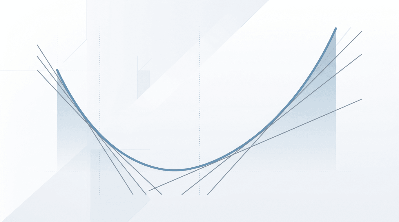
A function is said to be convex (or concave upward) on an interval if the line segment connecting any two points on the graph lies above or on the graph itself. Visually, a convex curve resembles a cup or a smile. It bends upward, meaning that as you move from left to right, the slope of the curve is increasing.

Another way to visualize this is through tangent lines: if you draw tangent lines to a convex curve at various points, the curve will lie entirely above these tangent lines.

Concavity (Concave Down)

Conversely, a function is said to be concave (or concave downward) on an interval if the line segment connecting any two points on the graph lies below or on the graph itself. Visually, a concave curve resembles a dome or a frown. It bends downward, meaning that as you move from left to right, the slope of the curve is decreasing.

For a concave curve, if you draw tangent lines at various points, the curve will lie entirely below these tangent lines.

Terminology Note: In pure mathematics and advanced optimization, the term "convex" is preferred for curves that open upward, while "concave" is preferred for curves that open downward. In introductory calculus, teachers often use "concave up" and "concave down" to avoid confusion. We will use these terms interchangeably to ensure complete clarity.

The Mathematical Test: The Second Derivative

How do we determine the concavity or convexity of a function algebraically? The answer lies in the second derivative of the function.

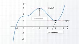
Let f(x) be a differentiable function. The first derivative, f'(x), represents the rate of change of the function (its slope). The second derivative, f''(x), is the derivative of the first derivative. Therefore, f''(x) represents the rate of change of the slope.

• If f''(x) > 0 for all x in an interval: The slope is increasing. This means the graph is bending upward, so the function is convex (concave up) on that interval.

• If f''(x) < 0 for all x in an interval: The slope is decreasing. This means the graph is bending downward, so the function is concave (concave down) on that interval.

What Happens When the Second Derivative is Zero?

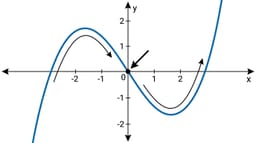
If f''(x) = 0 at a point, or if the second derivative does not exist at that point, this is a candidate for an inflection point. An inflection point is a point on the graph where the concavity changes from upward to downward, or vice versa.

It is important to note that f''(x) = 0 does not automatically guarantee an inflection point. For a point to be a true inflection point, the sign of f''(x) must change as you pass through that point.

A Step-by-Step Calculus Example

Let us analyze the cubic function f(x) = x^3 - 3x^2 + 2x to find its intervals of concavity and any inflection points.

1. Find the first derivative:
   Using the power rule, we get:
   f'(x) = 3x^2 - 6x + 2

2. Find the second derivative:
   Differentiating the first derivative gives:
   f''(x) = 6x - 6

3. Find where the second derivative is zero:
   Set f''(x) = 0:
   6x - 6 = 0
   6x = 6
   x = 1

4. Test the intervals:
   We now test the intervals around x = 1 (namely, x < 1 and x > 1) to see the sign of f''(x).
   

   • For x < 1 (e.g., x = 0): f''(0) = 6(0) - 6 = -6. Since this is negative, the function is concave down on the interval (-infinity, 1).

   • For x > 1 (e.g., x = 2): f''(2) = 6(2) - 6 = 6. Since this is positive, the function is concave up (convex) on the interval (1, infinity).

5. Identify the inflection point:
   Since the concavity changes at x = 1, this is a true inflection point. By plugging x = 1 back into the original function, we get f(1) = 1^3 - 3(1)^2 + 2(1) = 0. Thus, the inflection point is at (1, 0).

Physical and Scientific Applications

1. Kinematics and Motion in Physics

In physics, if we plot the position of an object over time, the graph's slope represents velocity (the first derivative). The acceleration of the object is the rate of change of velocity, which is the second derivative. Therefore, the concavity of a position-time graph directly tells us about the object's acceleration:

• A concave up position graph indicates positive acceleration (the object is speeding up in the positive direction or slowing down while moving backward).

• A concave down position graph indicates negative acceleration or deceleration (the object is slowing down or accelerating in the negative direction).

2. Optics and Light Behavior

In physics and optical engineering, lenses are classified based on their curvature:

• Convex Lenses: These lenses curve outward. They converge incoming parallel light rays to a single focal point. They are used in magnifying glasses, microscopes, and farsightedness correction.

• Concave Lenses: These lenses curve inward. They diverge incoming parallel light rays, making them spread out. They are used in peepholes, flashlights, and nearsightedness correction.

3. Economics: Diminishing Marginal Utility

In economics, production and utility functions are often analyzed using concavity. The concept of diminishing marginal utility states that as a person consumes more of a good, the additional satisfaction (utility) gained from each new unit decreases. This is represented by a function that is increasing but concave down. The slope is positive (more consumption means more total utility), but the second derivative is negative (the rate of increase is slowing down).

Key Takeaways

Understanding concavity and convexity allows us to describe the qualitative behavior of curves with extreme precision. Here are the core concepts to remember:

• Convexity (Concave Up): The curve bends upward like a cup; tangent lines lie below the curve; the second derivative is positive (f''(x) > 0).

• Concavity (Concave Down): The curve bends downward like a dome; tangent lines lie above the curve; the second derivative is negative (f''(x) < 0).

• Inflection Point: The point where a curve transitions between concave and convex, marked by a change in the sign of the second derivative.

• Real-world Relevance: These principles explain physical acceleration, the behavior of optical lenses, and economic trends of diminishing returns.