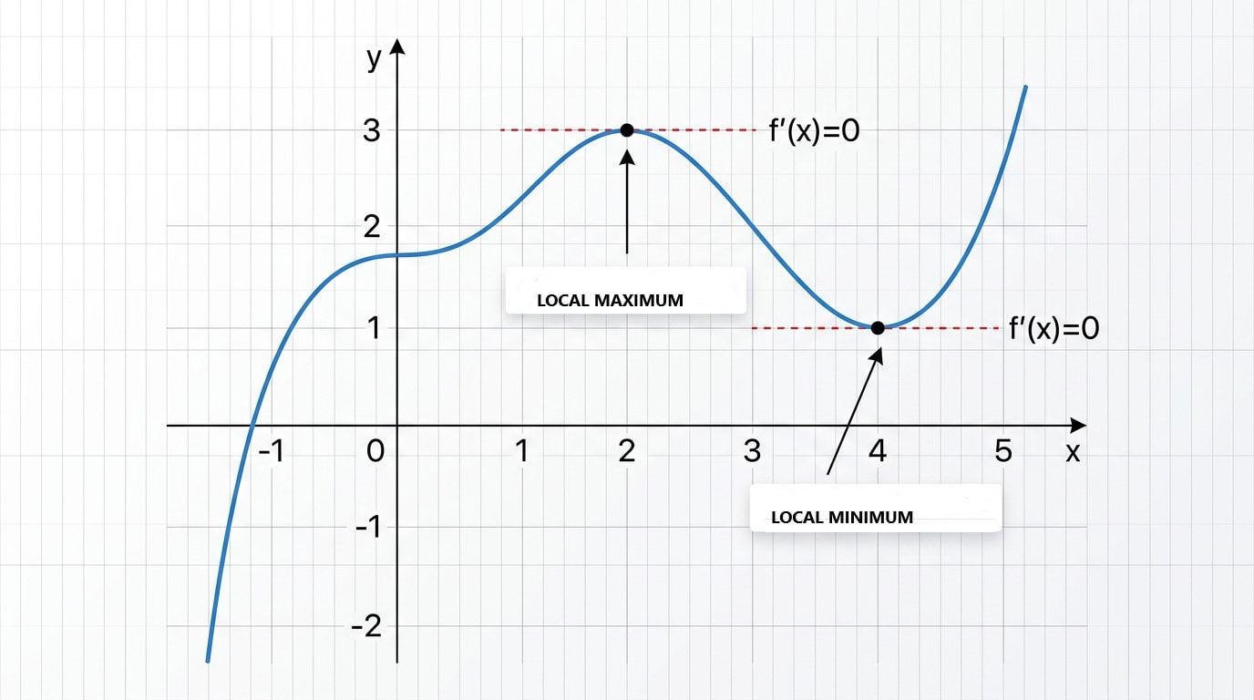
When we look at the natural world, we see a constant quest for balance, efficiency, and optimization. Bubbles form perfect spheres to minimize surface tension, rivers carve paths of least resistance, and physical systems naturally seek states of lowest energy. In mathematics, this universal search for the "highest" or "lowest" states is captured by the study of extremum points.
Extremum points—consisting of local maxima and local minima—are fundamental concepts in calculus and mathematical analysis. They allow us to analyze the behavior of functions, design optimal systems, and understand the physical laws governing our universe. In this comprehensive guide, we will explore what extremum points are, how they are defined mathematically, how to locate them using derivatives, and how they apply to real-world scientific phenomena.
What is an Extremum Point?
The word "extremum" (plural: extrema) comes from the Latin word for "extreme." In mathematics, an extremum point is a point where a function reaches its highest or lowest value within a specific region or over its entire domain.
To understand this conceptually, imagine walking along a mountainous terrain. As you hike, you will encounter peaks and valleys:
A Peak (Local Maximum): When you stand at the top of a hill, you are at the highest point in your immediate vicinity. Even if there are taller mountains far away, you are at a local high point.
A Valley (Local Minimum): When you stand at the bottom of a depression or basin, you are at the lowest point in your immediate surroundings. Even if there are deeper ocean trenches elsewhere, you are at a local low point.
In mathematical terms, we distinguish between two main types of extrema:
Local (Relative) Extrema: The highest or lowest values of a function within a specific, restricted interval.
Absolute (Global) Extrema: The absolute highest or lowest values of a function over its entire domain.
Our focus here is on local extrema—the local maxima and local minima that define the local structural behavior of a mathematical curve.
Rigorous Mathematical Definitions
To analyze these points scientifically, we must move beyond physical analogies and look at the formal definitions. Let f be a function defined on an interval I, and let c be a point within that interval.
1. Local Maximum
A function f has a local maximum at a point c if there exists an open interval containing c such that:
f(c) ≥ f(x) for all x in that open interval.
In plain terms, the output value f(c) is greater than or equal to any other output value in the immediate neighborhood of c.
2. Local Minimum
A function f has a local minimum at a point c if there exists an open interval containing c such that:
f(c) ≤ f(x) for all x in that open interval.
This means that the output value f(c) is less than or equal to any other output value in the immediate neighborhood of c.
How to Find Extremum Points: The Power of Derivatives
If we have the graph of a function, we can often spot the local maxima and minima visually. However, to find these points precisely and analytically, we rely on calculus—specifically, derivatives.
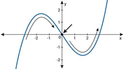
Recall that the derivative of a function, denoted as f'(x), represents the slope of the tangent line to the curve at any point x. At the very peak of a smooth hill (a local maximum) or the very bottom of a smooth valley (a local minimum), the tangent line is perfectly horizontal. A horizontal line has a slope of zero.
Critical Points: The Starting Search Area
According to Fermat's Theorem on Stationary Points, if a function f has a local extremum at c, and if the derivative exists at that point, then:
f'(c) = 0
This leads us to the concept of critical points. A critical point of a function f is a value c in the domain of f where either:
The derivative is zero: f'(c) = 0
The derivative is undefined: f'(c) does not exist
Important Note: While every local extremum occurs at a critical point, not every critical point is a local extremum. For example, consider the function f(x) = x³. Its derivative is f'(x) = 3x². At x = 0, the derivative is 0, making it a critical point. However, x = 0 is neither a local maximum nor a local minimum; it is an inflection point where the curve flattens out but continues to rise.
Testing Critical Points for Extrema
Once we have identified the critical points, we must test them to determine whether they are local maxima, local minima, or neither. Mathematicians use two primary tests for this purpose.
1. The First Derivative Test
The First Derivative Test examines the sign of the derivative (the slope of the curve) on either side of a critical point c:
From Positive to Negative: If f'(x) changes from positive to negative as you move from left to right through c, then f has a local maximum at c. (The function was climbing, reached the peak, and is now descending).
From Negative to Positive: If f'(x) changes from negative to positive as you move from left to right through c, then f has a local minimum at c. (The function was descending, reached the bottom, and is now climbing).
No Sign Change: If f'(x) does not change sign (remaining positive on both sides or negative on both sides), then c is not a local extremum.
2. The Second Derivative Test
The Second Derivative Test uses the concept of concavity (whether the graph curves upward like a cup or downward like a dome). The second derivative, f''(x), measures this concavity:
If f'(c) = 0 and f''(c) < 0, the curve is concave down (like a dome) at c. Therefore, c is a local maximum.
If f'(c) = 0 and f''(c) > 0, the curve is concave up (like a cup) at c. Therefore, c is a local minimum.
If f''(c) = 0, the test is inconclusive. You must revert to the First Derivative Test to make a determination.
Scientific and Physical Real-World Applications
1. Classical Physics and Potential Energy
In physics, physical systems naturally seek states of minimum energy. Consider a simple bowl with a marble inside:
Stable Equilibrium (Local Minimum): If the marble is at the bottom of the bowl, it is at a local minimum of gravitational potential energy. If you nudge it slightly, it will roll back toward the bottom. This is a stable state.
Unstable Equilibrium (Local Maximum): If you flip the bowl upside down and carefully balance the marble on top, it is at a local maximum of potential energy. A tiny nudge will cause it to roll away from the peak. This is an unstable state.
By finding the local minima of potential energy functions, physicists can predict the stable configurations of molecules, crystals, and mechanical structures.
2. Economics and Business Optimization
Businesses rely heavily on optimization models to make strategic decisions. By modeling real-world variables as mathematical functions, analysts can calculate critical thresholds:
Maximizing Revenue/Profit: Companies model their profit functions based on production volume and price. Finding the local maximum of the profit function tells the company exactly how many units to produce to achieve peak profitability.
Minimizing Cost: Supply chain networks design cost functions that incorporate transportation, labor, and material costs. Finding the local minimum of these functions helps minimize expenses.
3. Artificial Intelligence and Machine Learning
In modern computer science, machine learning models are trained using optimization algorithms like Gradient Descent. A model is given a "loss function" (or cost function) that measures how many errors it makes. The goal of the algorithm is to navigate the mathematical landscape of this loss function to find its local minimum, resulting in a highly accurate model with minimal errors.
Key Takeaways
Extremum points consist of local maxima (peaks) and local minima (valleys).
A local maximum is higher than any nearby point, while a local minimum is lower than any nearby point.
To locate these points analytically, we look for critical points where the first derivative f'(x) is zero or undefined.
We classify critical points using the First Derivative Test (observing changes in slope) or the Second Derivative Test (observing concavity).
Understanding local extrema is essential for solving real-world optimization problems in physics, economics, engineering, and data science.