In the study of calculus and mathematical analysis, few concepts are as fundamental and intuitive yet mathematically rigorous as continuity. When we first encounter graphs in algebra, we are often told that a continuous function is one whose graph can be drawn without lifting your pencil from the paper. While this visual analogy is excellent for building initial intuition, it falls short when we need to analyze complex mathematical models, prove theorems, or solve real-world engineering and economic problems.
To transition from intuitive understanding to mathematical mastery, we must establish the precise, rigorous conditions that define continuity at a point. In this comprehensive guide, we will break down the three essential conditions for continuity, explore how limits and function values interact, analyze piecewise functions, look at different types of discontinuities, and examine how these concepts apply to real-world scenarios like production costs and physical motion.
The Intuitive vs. The Rigorous Definition
Before diving into the technical conditions, let us contrast the informal idea of continuity with its formal counterpart. Informally, a continuous process is one that changes gradually without sudden jumps, breaks, or holes. For example, the growth of a tree, the warming of a cup of coffee, or the acceleration of a car are all continuous processes.
Mathematically, however, we cannot rely on visual inspectability. We need a definition based on limits and function values. A function is said to be continuous on an interval if it is continuous at every single point within that interval. Therefore, understanding continuity on a grand scale requires us to first understand continuity at a single, specific point.
The Three Essential Conditions for Continuity
For a function f(x) to be continuous at a specific point where x = c, it must satisfy three strict conditions. If even one of these conditions is violated, the function is discontinuous at that point.
The Definition of Continuity at a Point:
A function f(x) is continuous at x = c if and only if:
limx → c f(x) = f(c)
To fully comprehend this compact equation, we must unpack it into three distinct, chronological requirements:
Condition 1: The Function Must Be Defined at the Point
The first condition is that f(c) must exist. This means that the number c must lie within the domain of the function f(x). If you plug c into the function, it must yield a well-defined, real number output.
If the function is undefined at x = c (for example, due to division by zero, taking the square root of a negative number in real-valued functions, or a logarithmic argument being non-positive), the function cannot be continuous at that point. Visually, this often manifests as a hole or a vertical asymptote on the graph.
Condition 2: The Limit of the Function Must Exist as x Approaches c
The second condition is that the limit limx → c f(x) must exist. This requirement shifts our focus away from what is happening exactly at x = c to what is happening in the immediate neighborhood of c.
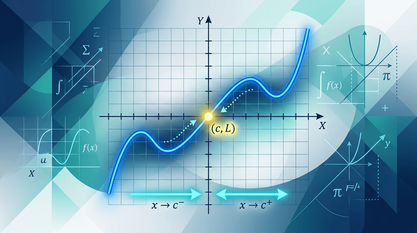
For a two-sided limit to exist, the left-hand limit and the right-hand limit must both exist and be equal to the same finite real number L:
Left-hand limit: limx → c− f(x) = L
Right-hand limit: limx → c+ f(x) = L
If the left-hand and right-hand limits do not match, or if the function approaches infinity as x approaches c, then the limit does not exist, violating this second condition.
Condition 3: The Limit and the Function Value Must Be Equal
The third and final condition is the bridge that unites the first two: limx → c f(x) = f(c). It is not enough for the function value to exist, and it is not enough for the limit to exist; they must be exactly the same value.
This condition ensures that the "expected" behavior of the function (represented by the limit as we approach c) perfectly matches the "actual" behavior of the function (represented by the value of the function at c). If they are different, the graph will have a point that is displaced or detached from the surrounding curve, creating a puncture or hole.
Visualizing Violations: Types of Discontinuity
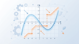
To reinforce these conditions, let us look at what happens when they are broken. These violations are classified into three primary types of discontinuities:
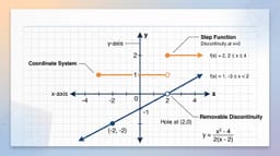
Removable Discontinuity (Hole): This occurs when the limit exists, but either the function is not defined at that point, or the function's value does not equal the limit. It is called "removable" because you could make the function continuous simply by redefining or "filling in" the single point.
Example: f(x) = (x2 - 4) / (x - 2) at x = 2.Jump Discontinuity: This occurs when the left-hand limit and the right-hand limit both exist as finite numbers, but they are not equal. The graph literally "jumps" from one height to another.
Example: The step function or piecewise functions where different formulas meet at a boundary.Infinite Discontinuity: This occurs when one or both of the one-sided limits go to positive or negative infinity. This typically corresponds to a vertical asymptote.
Example: f(x) = 1 / x at x = 0.
Analyzing Continuity in Piecewise Functions
Piecewise functions are the perfect testing ground for analyzing continuity because they are built from different formulas over different intervals. The boundaries where these formulas transition are called critical points, and they require careful investigation.
Let us consider the following piecewise function:
g(x) =
2x + 3, if x < 1
k, if x = 1
x2 + 4, if x > 1
Let us determine if there is a value of k that makes the function continuous at x = 1 by testing our three conditions:
Step 1: Check the function value. By definition, g(1) = k. Condition 1 is satisfied as long as k is a real number.
Step 2: Check the limit. We must evaluate the left-hand and right-hand limits as x approaches 1.
Left-hand limit: limx → 1− (2x + 3) = 2(1) + 3 = 5
Right-hand limit: limx → 1+ (x2 + 4) = (1)2 + 4 = 5
Since both one-sided limits are equal to 5, the two-sided limit exists and limx → 1 g(x) = 5. Condition 2 is satisfied.
Step 3: Set the limit equal to the function value. For the function to be continuous, we must satisfy Condition 3: limx → 1 g(x) = g(1). Therefore, we set 5 = k.
By choosing k = 5, we satisfy all three conditions, making the function g(x) continuous at x = 1.
Key Mathematical Propositions Regarding Continuity
Mathematicians have developed several powerful propositions and theorems that allow us to determine the continuity of complex functions without having to perform the three-step limit test every time:
Algebra of Continuous Functions: If f(x) and g(x) are both continuous at x = c, then their sum (f + g), difference (f - g), and product (f · g) are also continuous at x = c. Their quotient (f / g) is also continuous at x = c, provided that g(c) ≠ 0.
Continuity of Basic Functions: Polynomials, exponential functions, logarithmic functions, trigonometric functions, and rational functions are continuous at every point within their respective domains.
Composite Function Theorem: If g is continuous at c and f is continuous at g(c), then the composite function (f ˆ g)(x) = f(g(x)) is continuous at x = c.
Intermediate Value Theorem (IVT): If a function f is continuous on a closed interval [a, b], then for any value M strictly between f(a) and f(b), there exists at least one value c in the interval (a, b) such that f(c) = M. This theorem is crucial for proving the existence of roots and solving physical equations.
Real-World Applications of Continuity
Continuity is not just a theoretical tool; it is a vital framework for modeling real-world phenomena. In physical systems, nature generally operates continuously, whereas human systems (like economics and digital technology) often introduce discontinuities.
Example 1: Production Costs and Economy of Scale
In business and economics, the cost of manufacturing a product can be modeled as a function of the quantity produced. Let us analyze two scenarios:
Discontinuous Pricing (Bulk Discount Steps): A company might sell raw materials where buying under 100 kg costs 8/kg. This pricing structure creates a jump discontinuity at x = 100. A tiny increase in order size from 99.9 kg to 100 kg results in a sudden, sharp drop in total cost.
Continuous Marginal Costing: Modern automated production plants model costs using continuous functions where setup costs, material consumption, and energy efficiency scale smoothly. A continuous cost function allows managers to use derivatives and optimization algorithms (like finding the exact point of maximum profit), which require continuity to function correctly.
Example 2: Physical Motion and Kinematics
In physics, the position of an object over time must be a continuous function. An object cannot instantly teleport from position A to position B; it must pass through every intermediate point. Similarly, while velocity can change rapidly (such as during a collision), the velocity curve of a real physical object is continuous due to inertia and the finite nature of forces. Modeling these physical systems using continuous functions allows engineers to design safe vehicles, bridges, and aerospace trajectories.
Key Takeaways
Continuity at a point requires three conditions: the function value must exist, the limit must exist, and they must be equal.
Limits look at the behavior near a point, while the function value looks at the behavior exactly at that point. Continuity is the perfect agreement between the two.
Understanding the types of discontinuities (removable, jump, and infinite) helps diagnose where and why mathematical models fail.
Real-world models, from physics to economics, rely on continuity to make predictions, optimize processes, and apply calculus tools.