If you have ever watched a speedometer in a car fluctuate as you press the gas pedal, you have experienced a fundamental puzzle of the physical universe: instantaneous rate of change. At any exact millisecond, how fast are you moving? Standard speed calculations require a distance traveled over a span of time. But an "instant" has no duration. How can we measure speed when time does not pass?
This physical paradox is mirrored perfectly in geometry. If you have a curved line on a graph, how do you measure its steepness at one exact, single point? The answer to both the physical and geometric questions lies in a single, revolutionary concept: the slope of the tangent line. This article will guide you through the journey of understanding, defining, proving, and applying this cornerstone of calculus.
1. The Geometric Intuition: Secant to Tangent
To understand the slope of a tangent line, we must first look at a line we already know how to measure: the secant line. In geometry, a secant line is a straight line that passes through at least two distinct points on a curve.
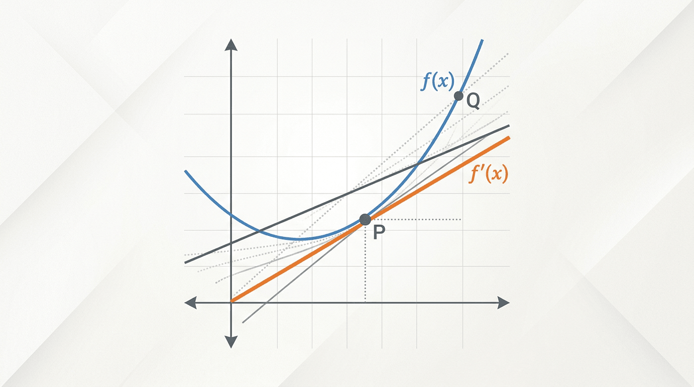
Let us assume we have a continuous function represented by y = f(x). We want to find the steepness of this curve at a specific point, let's call it P(x, f(x)). If we choose another point nearby on the curve, say Q(x + h, f(x + h)), where h represents a small horizontal distance from x, we can easily draw a secant line through P and Q.
The slope of this secant line (which we will call msec) is given by the classic algebra formula for slope (rise over run):
msec = [f(x + h) - f(x)] / [(x + h) - x] = [f(x + h) - f(x)] / h
This ratio is known as the difference quotient. It represents the average rate of change of the function over the interval [x, x + h]. But what happens if we want the slope at exactly point P?
We imagine point Q sliding along the curve closer and closer to point P. As Q approaches P, the horizontal distance h shrinks toward zero. The secant line begins to pivot, aligning itself more closely with the curve at point P. At the exact moment when h reaches zero, the two points merge into one. The line that once crossed two points now grazes the curve at exactly one point. This is the tangent line, and its slope is the instantaneous rate of change of the curve at point P.
2. Formalizing the Slope with Limits
We cannot simply plug h = 0 into our secant slope formula because that would result in division by zero, which is mathematically undefined. To resolve this, we use the concept of a limit. The limit allows us to observe the value that the difference quotient approaches as h gets infinitely close to zero, without ever actually letting h equal zero.
Therefore, the slope of the tangent line (mtan), which is also defined as the derivative of the function at x (denoted as f'(x)), is formally written as:
f'(x) = limh → 0 [f(x + h) - f(x)] / h
This limit is the foundational definition of the derivative. If this limit exists, we say the function is differentiable at x, and the resulting value is the precise slope of the tangent line at that point.
3. How Combined Functions Affect the Slope of the Tangent Line
In real-world applications, physical systems are rarely modeled by simple, isolated functions. They are often combinations of multiple functions through addition, subtraction, multiplication, division, and composition. To find the slope of the tangent line for these complex systems, we must understand how their individual component slopes behave.
Let us rigorously derive these relationships using the limit definition of the tangent slope.
A. The Sum and Difference Rules
Suppose we have a new function that is the sum of two differentiable functions: u(x) = f(x) + g(x). What is the slope of the tangent line of u(x)?
We set up the limit definition for u'(x):
u'(x) = limh → 0 [u(x + h) - u(x)] / h
Substitute u(x) = f(x) + g(x) into the equation:
u'(x) = limh → 0 [(f(x + h) + g(x + h)) - (f(x) + g(x))] / h
Rearranging the terms in the numerator allows us to group the f terms and g terms together:
u'(x) = limh → 0 [ (f(x + h) - f(x)) + (g(x + h) - g(x)) ] / h
Using the limit law which states that the limit of a sum is the sum of the limits, we can separate the fractions:
u'(x) = limh → 0 [f(x + h) - f(x)] / h + limh → 0 [g(x + h) - g(x)] / h
We recognize these two separate limits as the definitions of f'(x) and g'(x). Thus, we arrive at our generalization:
(f + g)'(x) = f'(x) + g'(x)
The same logic applies to subtraction. This proves that the slope of the tangent line of a combined sum/difference function is simply the sum/difference of the individual slopes of the tangent lines.
B. The Product Rule
Now, let's look at a product of two functions: p(x) = f(x) · g(x). It is a common mistake to assume that the slope of a product is simply the product of the slopes. Let us use the limit definition to find the true pattern.
p'(x) = limh → 0 [f(x + h)g(x + h) - f(x)g(x)] / h
To solve this limit, we use a classic mathematical technique: adding and subtracting the same term, f(x + h)g(x), in the numerator. This does not change the value of the expression, but it allows us to factor terms:
p'(x) = limh → 0 [f(x + h)g(x + h) - f(x + h)g(x) + f(x + h)g(x) - f(x)g(x)] / h
Now, let us group and factor the numerator:
p'(x) = limh → 0 [ f(x + h) · (g(x + h) - g(x)) + g(x) · (f(x + h) - f(x)) ] / h
Splitting this into two separate limits yields:
p'(x) = limh → 0 [f(x + h) · (g(x + h) - g(x)) / h] + limh → 0 [g(x) · (f(x + h) - f(x)) / h]
As h → 0, the term f(x + h) becomes f(x) because f is continuous. The other parts of the expression transform directly into the limit definitions of derivatives:
(f · g)'(x) = f(x)g'(x) + g(x)f'(x)
This elegant rule shows that the slope of the tangent line of a product function depends not only on the slopes of the individual functions but also on the values of those functions at that point.
C. The Quotient Rule
What about a quotient of two functions: q(x) = f(x) / g(x), where g(x) ≠ 0? Let's apply the limit definition:
q'(x) = limh → 0 [ (f(x + h) / g(x + h)) - (f(x) / g(x)) ] / h
First, we find a common denominator for the terms in the numerator:
q'(x) = limh → 0 [ (f(x + h)g(x) - f(x)g(x + h)) / (g(x + h)g(x)) ] / h
We can rewrite this by pulling the denominator to the side:
q'(x) = limh → 0 [ 1 / (g(x + h)g(x)) ] · limh → 0 [ (f(x + h)g(x) - f(x)g(x + h)) / h ]
For the second limit, we use our trick of adding and subtracting a term, in this case f(x)g(x), in the numerator:
limh → 0 [ (f(x + h)g(x) - f(x)g(x) + f(x)g(x) - f(x)g(x + h)) / h ]
Factor out g(x) from the first two terms and -f(x) from the last two terms:
limh → 0 [ g(x) · (f(x + h) - f(x)) / h - f(x) · (g(x + h) - g(x)) / h ]
Evaluating the limits as h → 0, we get:
g(x)f'(x) - f(x)g'(x)
Combining this with the first part, limh → 0 [ 1 / (g(x + h)g(x)) ] = 1 / [g(x)]2, we get the complete quotient rule:
(f / g)'(x) = [ f'(x)g(x) - f(x)g'(x) ] / [g(x)]2
D. The Chain Rule (Composition of Functions)
Finally, let us consider a composite function: y = f(g(x)). This represents a situation where one process feeds directly into another. How do we find the slope of the tangent line of f(g(x))?
Let u = g(x). A change in x, denoted by Δx, causes a change in u, denoted by Δu, which in turn causes a change in y, denoted by Δy.
We can write the average rate of change as a product of two ratios:
Δy / Δx = (Δy / Δu) · (Δu / Δx)
As Δx → 0, the change in the intermediate function Δu also approaches 0 (assuming g is continuous). Taking the limit of both sides as the changes approach zero gives us the derivative:
limΔx → 0 (Δy / Δx) = limΔu → 0 (Δy / Δu) · limΔx → 0 (Δu / Δx)
This yields the famous Chain Rule:
(f(g(x)))' = f'(g(x)) · g'(x)
In terms of tangent slopes, this means that the slope of the composite function is the product of the slope of the outer function (evaluated at the inner function's value) and the slope of the inner function.
4. Evaluating the Usefulness of These Proofs
Why do mathematicians spend time proving these rules with limits instead of just memorizing them? There are several reasons why this process is incredibly useful:
Guaranteed Truth: Using the limit definition ensures that these rules are not assumptions. They are mathematical truths derived from the fundamental definition of space and change.
Efficiency: While the limit definition is the ultimate source of truth, calculating limits for complex equations every single time is incredibly time-consuming. These derived rules act as "shortcuts" that allow us to find the slope of any tangent line in seconds.
Structural Insight: Proving these rules shows us how different mathematical operations scale. For instance, the product rule shows us that the rate of change of an area (length times width) depends on both the changing length and the changing width simultaneously.
5. Real-World Applications: Why the Tangent Slope Matters
The slope of the tangent line is not just a theoretical concept on a graph. It is the language of modern science and engineering. Here are a few ways it is applied across different disciplines:
A. Physics: Motion and Mechanics
If you graph the position of an object over time, the slope of the secant line between two times gives you the average velocity. However, the slope of the tangent line at a specific second gives you the instantaneous velocity—the exact speed and direction of the object at that precise moment. Taking the tangent slope of the velocity curve gives you acceleration.
B. Chemistry: Rates of Reaction
In a chemical reaction, the concentration of reactants decreases over time. If you plot the concentration of a reactant on a graph, the slope of the tangent line at any point tells you the instantaneous reaction rate. This allows chemists to understand exactly how fast molecules are colliding and reacting at any given second.
C. Economics: Marginal Analysis
In business, profit, cost, and revenue are modeled as functions of the quantity of goods produced. The slope of the tangent line on a cost curve represents the marginal cost—the cost of producing exactly one more unit. By analyzing these tangent slopes, economists can determine the exact level of production that maximizes a company's profit.
6. Key Takeaways
Understanding the slope of the tangent line is the key that unlocks the door to calculus. Here are the core concepts to remember:
The slope of a tangent line represents the instantaneous rate of change of a function at a single point.
It is found by taking the limit of the slope of a secant line as the distance between the two points approaches zero.
Using the limit definition, we can prove rules (Sum, Product, Quotient, and Chain rules) that allow us to easily calculate the tangent slope of complex, combined functions.
These slopes are used in physics, chemistry, economics, and engineering to measure real-time changes in our dynamic world.
By mastering how to find and interpret the slope of the tangent line, you gain the ability to analyze and predict how things change, move, and flow throughout the universe.