Within this profound branch of science, the definite integral serves as one of its twin pillars, alongside the derivative. While derivatives analyze rates of change at a precise moment, definite integrals solve the inverse and equally vital problem: the accumulation of quantities over a continuous interval.
Whether you are calculating the total distance traveled by an accelerating spacecraft, determining the work done by a variable magnetic field, or modeling the distribution of probability in quantum mechanics, the definite integral is the mathematical engine that drives these calculations. This comprehensive guide will explore what a definite integral is, dissect its geometric and physical meanings, trace its rigorous mathematical definition, and demonstrate how to calculate it using the Fundamental Theorem of Calculus.
The Intuitive Core: Area Under a Curve
To understand the definite integral, we must first look at a fundamental geometric challenge. Since antiquity, mathematicians have known how to calculate the areas of shapes with straight edges, such as rectangles, triangles, and polygons. Even the area of a circle was solved using clever geometric approximations.
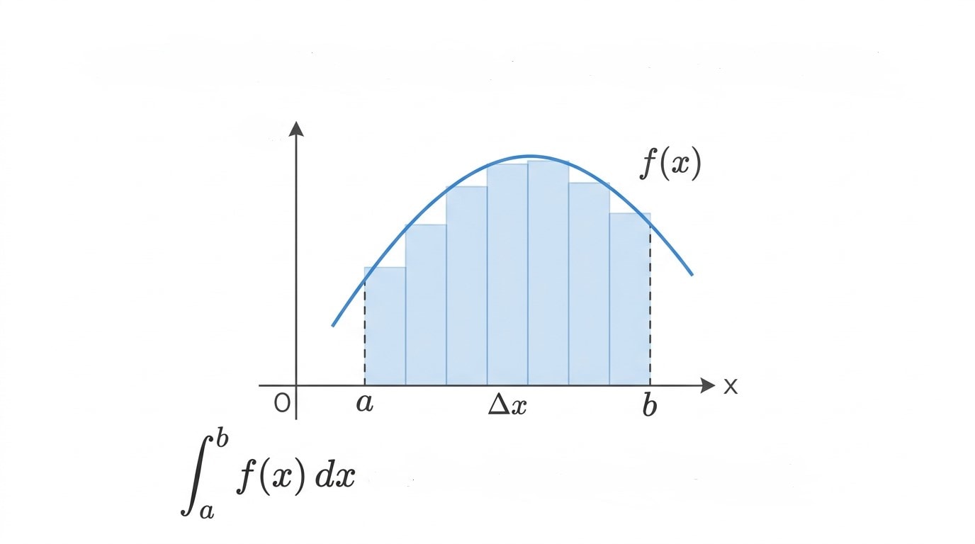
However, what happens when we want to find the area under an arbitrary curve, such as the graph of a function f(x) between two points a and b on the horizontal axis? This is where standard geometry fails, and where the definite integral begins.
Geometric Definition: Geometrically, the definite integral of a continuous, non-negative function f(x) over an interval [a, b] represents the exact area bounded by the graph of the function, the x-axis, and the vertical lines x = a and x = b.
If the function dips below the x-axis, the definite integral does not simply calculate absolute physical area; instead, it measures the signed area. Areas above the x-axis are treated as positive values, while areas below the x-axis are treated as negative values. The definite integral calculates the net sum of these positive and negative regions.
The Rigorous Definition: Riemann Sums
How do we turn the intuitive concept of "area" under a curved line into a rigorous mathematical definition? The answer lies in the work of the German mathematician Bernhard Riemann, who formalized the process using what we now call Riemann Sums.
The strategy is elegant: if we cannot calculate the area of a curved shape directly, we can approximate it using shapes we do know how to measure—rectangles.
Step 1: Partitioning the Interval
First, we take the closed interval [a, b] on the x-axis and divide it into n smaller subintervals. We can define these division points as:
a = x0 < x1 < x2 < ... < xn-1 < xn = b
The width of each subinterval is denoted by Δxi = xi - xi-1. For simplicity, we often make all subintervals of equal width, which means:
Δx = (b - a) / n
Step 2: Constructing the Rectangles
For each subinterval, we choose a sample point, which we will call xi*. This point can be chosen anywhere within the subinterval (for example, the left endpoint, the right endpoint, or the midpoint).
We then construct a rectangle over each subinterval. The width of the rectangle is Δx, and its height is the value of the function at our chosen sample point, f(xi*). The area of a single rectangle is therefore:
Area of one rectangle = f(xi*) · Δx
Step 3: Summing the Rectangles
By adding the areas of all n rectangles together, we obtain an approximation of the total area under the curve. This sum is the Riemann Sum:
Riemann Sum = ∑i=1n f(xi*) Δx
Step 4: Taking the Limit to Infinity
As we increase the number of rectangles (n) toward infinity, the width of each individual rectangle (Δx) shrinks toward zero. The approximation becomes increasingly accurate, eventually eliminating all error.
The definite integral is defined as the limit of this Riemann sum as the number of subintervals approaches infinity:
∫ab f(x) dx = limn → ∞ ∑i=1n f(xi*) Δx
In this elegant notation, introduced by Gottfried Wilhelm Leibniz:
The integral symbol ∫ is an elongated "S", standing for "summa" (sum).
The numbers a and b are the limits of integration (the starting and ending points).
f(x) is the integrand (the function being integrated).
dx represents an infinitely small change in x, replacing the discrete Δx of the Riemann sum.
The Fundamental Theorem of Calculus: The Great Bridge
Calculating limits of Riemann sums manually is incredibly difficult and tedious for all but the simplest functions. Fortunately, the Fundamental Theorem of Calculus (FTC) establishes a brilliant shortcut by linking integration directly to differentiation.
The theorem consists of two parts, but the second part is what allows us to evaluate definite integrals with ease:
The Fundamental Theorem of Calculus (Part 2): If f(x) is a continuous function on the closed interval [a, b], and F(x) is any antiderivative of f(x) (meaning that F'(x) = f(x)), then:
∫ab f(x) dx = F(b) - F(a)
This means that to find the definite integral, we do not need to construct millions of rectangles. We simply need to find the antiderivative of our function, plug in the upper limit b, plug in the lower limit a, and subtract the two results. This discovery revolutionized science and engineering, transforming complex physical calculations into simple algebraic exercises.
Essential Properties of Definite Integrals
Definite integrals follow several fundamental algebraic rules that make them highly versatile tools for analysis:
Linearity (Constant Multiple Rule): You can pull a constant factor out of the integral:
∫ab c · f(x) dx = c ∫ab f(x) dxLinearity (Sum/Difference Rule): The integral of a sum is the sum of the integrals:
∫ab [f(x) ± g(x)] dx = ∫ab f(x) dx ± ∫ab g(x) dxInterval Additivity: You can split an integral over a single interval into two adjacent intervals:
∫ab f(x) dx + ∫bc f(x) dx = ∫ac f(x) dxZero Width Interval: If the upper and lower limits are equal, the area is zero:
∫aa f(x) dx = 0Reversing Limits: Swapping the limits of integration negates the result:
∫ba f(x) dx = -∫ab f(x) dx
A Step-by-Step Calculation Example
Let us put theory into practice by evaluating a concrete definite integral:
Problem: Evaluate ∫13 (3x2 + 2x) dx
Step 1: Find the antiderivative.
Using the power rule for integration, we find the general antiderivative F(x) of the function f(x) = 3x2 + 2x:
F(x) = x3 + x2
Step 2: Apply the Fundamental Theorem of Calculus.
We need to compute F(3) - F(1).
First, calculate F(3):
F(3) = (3)3 + (3)2 = 27 + 9 = 36
Next, calculate F(1):
F(1) = (1)3 + (1)2 = 1 + 1 = 2
Step 3: Subtract the values.
F(3) - F(1) = 36 - 2 = 34
Thus, the value of the definite integral is 34. This is the exact net area under the curve y = 3x2 + 2x from x = 1 to x = 3.
Applications in Physics and Science
1. Kinematics: Position from Velocity
If an object moves along a straight line with a variable velocity v(t), its change in position (displacement) from time t = a to t = b is the definite integral of its velocity function:
Displacement = ∫ab v(t) dt
2. Classical Mechanics: Work Done by a Variable Force
In physics, work is defined as force multiplied by distance. However, if the force changes as the object moves (like stretching a spring), we must integrate the variable force function F(x) over the distance interval [a, b]:
Work = ∫ab F(x) dx
3. Probability Theory: Continuous Distributions
In statistics and quantum physics, the probability of an event occurring within a continuous range of values [a, b] is calculated by integrating a Probability Density Function (PDF), P(x):
Probability = ∫ab P(x) dx
Key Takeaways
The definite integral represents the accumulated net signed area under a curve over a specific interval [a, b].
It is mathematically defined as the limit of Riemann sums as the width of the approximating rectangles approaches zero.
The Fundamental Theorem of Calculus connects integration to differentiation, allowing us to evaluate integrals using antiderivatives.
It is a vital mathematical tool used across physics, engineering, chemistry, and statistics to model real-world accumulation.